The transition metal mercury has many exciting properties; for example, it is the only known metal that is liquid at room temperature, hence its use in thermometers. Other common applications are in energy-saving lamps and dental amalgam fillings. In centuries past, inorganic mercury compounds such as mercury(II) chloride were used in wood preservation. For the determination of total mercury content in wood, a very sensitive method using microwave digestion and cold vapor inductively coupled plasma-optical emission spectrometry (ICP-OES) was developed in which a detection limit in dried wood material of 3.41 μg/kg was achieved. Part 1 of this article describes the ICP-OES method used to determine total mercury content in waste wood. Part 2 will explore the role of inductively coupled plasma-mass spectrometry (ICP-MS) in mercury determination.
Mercury characteristics and applications
Until the middle of the last century, an economically important application of mercury was wood treatment with the sublimate mercury(II) chloride. John Howard Kyan invented a procedure called “kyanizing” that was patented in 1832 and was used for the impregnation of railroad ties, telegraph poles, and construction timber.1 Wood treatment using mercury(II) chloride provided very effective wood protection,2 but its application was highly controversial due to the health implications to humans.1 For example, waste wood such as disused railroad ties, telegraph poles, and wood from refurbished buildings may cause environmental pollution, and mercury may enter the human food chain.
In addition to inorganic bound mercury, organic mercury compounds were very important for their application in wood protection, but in particular for their use as fungicides3–5 and as additives in paints to protect against mold.6 In agricultural practices, the use of organic mercury compounds in Europe and other countries was discontinued in 1970.3
Despite its wide fields of application, there is great concern about mercury because of its high toxicity and resulting health damages to organisms. Depending on its binding form, mercury poisoning may cause damage to the liver, kidneys, brain, and especially the central nervous system.7,8 Well-known examples of environmental and industrial mercury poisoning in large areas are the occurrence of Minamata disease in Japan in the 1950s,9–11 and catastrophic mercury poisoning in Iraq in the 1970s.4
Mercury determination using ICP-OES, atomic absorption spectroscopy (AAS), and atomic fluorescence spectroscopy (AFS)
One of the first scientists to develop a method to detect minute amounts of mercury using a microscope was Alfred Stock, who himself suffered from chronic mercury poisoning and was thus aware of its toxic effects on human health.12 Over the years, new analytical techniques were established and detection limits decreased.13–15 Today, a multitude of important spectroscopic techniques are available, including ICP-OES,16 AAS, and AFS.17
The latter techniques are often combined with mercury cold vapor generation to avoid matrix effects and lower detection limits.18–20 This results in higher sensitivity, selectivity, and detection limits.21,22 Furthermore, ICP-MS is becoming more important in this context,23,24 as will be discussed in Part 2 of this article.
Experimental
Chemicals and reagents
The calibration, sample, and rinsing solutions were prepared using the following reagents: ultrapure water, Suprapur® nitric acid (65%, v/v), and Suprapur hydrochloric acid (30%, v/v) (Merck, Darmstadt, Germany); ICP mercury standard solution was also from Merck. Mercury cold vapor was generated with a reducing agent consisting of sodium tetrahydridoborate (≥98.0%) from Sigma Aldrich (Steinheim, Germany) and sodium hydroxide (≥97.0%) from Fluka (Buchs, Switzerland). For method validation, the reference wood ERM-CD100 containing 0.60 ± 0.14 mg/kg Hg from the German Federal Institute for Materials Research and Testing (BAM, Berlin, Germany) was used. In addition, 43 real wood samples of different origin, age, and degree of treatment were analyzed.
Instrumentation and parameters
Microwave-assisted digestion was performed using the Mars 5 Microwave Accelerated Reaction System with XP1500 vessels (vol. 50 mL, max. 55 bar) from CEM (Kamp-Lintfort, Germany). Magnetic stirrers from VWR (Darmstadt, Germany) with an elliptical shape and dimensions of 15 × 6 mm were made of PTFE and provided optimal mixing during the digestion. The cold vapor was generated using a gas–liquid separator and analyzed with the ICP-OES iCAP 6500 from Thermo Fisher Scientific (Dreieich, Germany) using the following parameters of argon plasma: rinsing and analysis pump rate of 25 U/min, stabilization time of 10 sec, radiofrequency power of 1150 W, auxiliary gas flow rate of 0.50 L/min, nebulizer gas flow of 0.60 L/min, and cooling gas flow of 12 L/min. The measurements were performed in axial view with three replicates at the emission line of 184.95 nm.
For automated sample introduction using the ASX-260 autosampler from Cetac (Omaha, NE), the rinsing time was set to 70 sec. The reducing agent consisted of 1.25 g sodium tetrahydridoborate (conc. 0.5%) and 1 g sodium hydroxide in a volumetric flask (vol. 250 mL) filled with ultrapure water. Classical ICP-OES analysis was performed using the following parameters: rinsing and analysis pump rate of 50 U/min, stabilization time of 5 sec, radiofrequency power of 1150 W, auxiliary gas flow rate of 0.50 L/min, nebulizer gas flow of 0.50 L/min, and cooling gas flow of 12 L/min. Each measurement was performed in axial view with three replicates at the emission line of 184.95 nm and a rinse time of 40 sec.
Standard and sample preparation
Figure 1 – Selected wood samples in different stages of sample pretreatment. The raw wood material was splintered into pieces using a ceramic scalpel and dried to constant weight at room temperature. To increase the surface, the wood chips were milled for 3 min at 95% power in the MM2000 ball mill from Retsch (Haan, Germany) using ceramic containers and balls. Figure 1 shows a selection of real wood samples in various stages of sample pretreatment. To 250–350 mg of the milled samples, 8 mL of nitric acid or aqua regia was added. Predigestion was performed over a period of 20 min with open vessels.
The basic microwave digestion procedure consisted of a temperature–time ramp for 20 min with a final temperature of 180 °C (356 °F) held for 20–30 min. The power was dependent on the number of vessels; for more than six vessels 1200 W were used. At each digestion run, one blank sample was included. After the digestion, the samples were cooled to room temperature. The clear sample solutions were transferred to a volumetric flask (vol. 100 mL) and filled with ultrapure water. The final acid concentration was 8% (v/v). The calibration solutions were prepared in nitric acid or aqua regia (concentration 8%, v/v) with Hg concentrations of 0.05–1.0 μg/L for cold vapor ICP-OES and 1–50 μg/L for classical ICP-OES. For cold vapor generation from samples in nitric acid, hydrochloric acid was added to a final concentration of 10% (v/v). The sample and calibration solutions were prepared and stored in vessels of polyethylene or polypropylene.
Results and discussion
The reference wood (Hg content: 0.46–0.74 mg/kg) was used to perform various validation experiments. For each microwave digestion procedure, repeatability testing was performed. The recovery rate, limit of detection (LOD), and limit of quantitation (LOQ) were determined. Finally, real wood samples from different origins were analyzed. The data evaluation was done according to Horwitz,25 who defines the within-laboratory coefficient of variation (CV) as usually one-half to two-thirds of between-laboratory CV, depending on the analyte concentration. In the case of Hg in a concentration of 0.6 mg/kg, the within-laboratory CV should not exceed 11.52%, which was attained in all experiments.
Repeatability testing and recovery rate
Using the reference wood, 34 samples were digested with aqua regia and 32 samples with nitric acid. All measurement results followed a normal distribution (determined by the David test), corresponded with the Hg content in the reference wood, and fulfilled the Horwitz criterion. The results of the aqua regia method showed a slightly higher CV and a higher recovery rate compared to the nitric acid method. According to Kromidas,26 a recovery rate is acceptable if the measured value is less from 100 than the fourfold of the CV. The recovery rates of the aqua regia method fulfilled this criterion; the nitric acid method resulted in lower recovery rates (see Table 1). The results of both methods are compared in Figure 2.
Table 1 – Results of repeatability testing and recovery rates for two microwave digestion methods
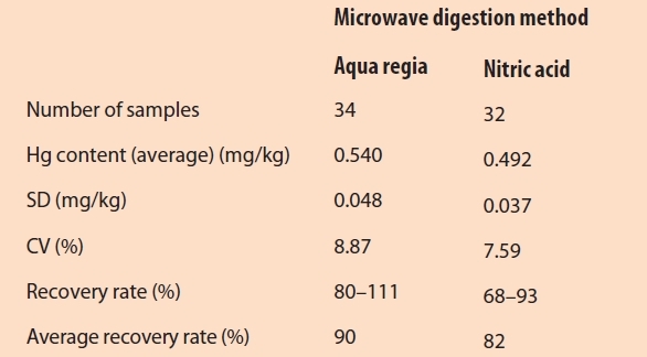
 Figure 2 – Comparison of two microwave digestion methods using Box-Whisker-Plots (the gray shaded area shows the interval of the expected value of the reference material).
Measurement precision, limit of detection, and limit of quantitation
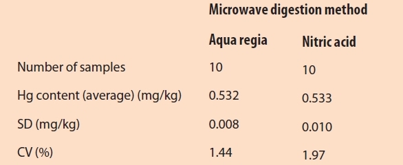
The measurement precision was determined with 10 measurements of the same sample for each digestion method. The CV values were lower than 2%, but by using aqua regia, the SD and CV were slightly lower than with nitric acid (see Table 2). The LOD and the LOQ were determined with measurements of 10 blank samples with aqua regia and the following equation26:
For the measurement solutions, the values of LOD and LOQ were 8.52 ng/L and 17.41 ng/L; in wood samples (dried matter) the values were 3.41 μg/ kg and 6.96 μg/kg.
Table 2 – Measurement precision for two microwave digestion methods
Comparison to classic ICP-OES using a spray chamber
Additionally, the CV of the ICP-OES method was compared with classic ICP-OES using a spray chamber. The recovery rates were 81–108% (average 96%) and the measurement precision shows an SD of 0.04 mg/kg and CV of 5.51%. The values of LOD and LOQ were significantly higher than for the cold vapor ICP-OES method. In the solutions the values of LOD and LOQ were 0.38 μg/L and 1.02 μg/L; in wood material, the values of 0.15 mg/kg and 0.41 mg/kg were determined.
Real wood sample analysis
Real wood samples were analyzed using the method presented. This included natural wood from the surrounding territory, i.e., wood from trees in a local city park and nearby streets; timber from sources such as from transport pallets, wooden floor boards, or old window frames; as well as treated wood such as roof beams, railroad ties, and utility and telephone poles. All samples were prepared using the aqua regia microwave digestion method. The analysis was performed using ICP-OES with mercury cold vapor and was compared with classical ICPOES. Table 3 shows the results for selected wood samples with a significant Hg content.
Table 3 – Total mercury content of selected real wood samples from different origins
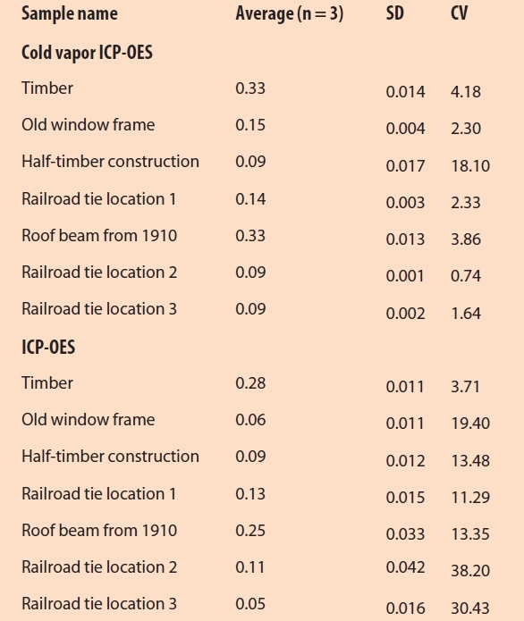
In general, the ICP-OES method using mercury cold vapor enabled very sensitive determination of total mercury. For the majority of samples, the measured CV values were significantly lower than the classic ICP-OES method. Figure 3 compares the total mercury content of selected wood samples determined using both techniques.
 Figure 3 – Comparison of cold vapor ICP-OES and classical ICP-OES using a spray chamber to determine total mercury content of selected wood samples of different origins.
Conclusion
For the determination of the total mercury content in waste wood, a very sensitive and fast method using cold vapor ICP-OES offered a limit of detection of 3.41 μg/kg in dried wood material. In comparison to classic ICP-OES, the LOD was reduced by around 97–98%. Sample preparation was done using microwave digestion with two acid compositions. Optimal results were achieved using aqua regia. Classic ICP-OES does not usually reach this low detection limit. Although cold vapor ICP-OES is a single-element method, easy modification of the instrument by removing the gas–liquid separator and installing the spray chamber enabled multielement measurements.
References
- Moll, F. Angew. Chem. 1913, 26(67), 459–63.
- Nowak, A. Eur. J. Wood and Wood Prod. 1952, 10(1), 12–15.
- Jitaru, P.; Adams, F. J. Phys. IV 2004, 121, 185–93.
- Bakir, F.; Damliji, S.F. et al. Science 1973, 181(4096), 230–41.
- Tatton, J.O.; Wagstaffe, P. J. Chromatogr. 1969, 44(2), 284–9.
- Sunderland, E.M.; Chmura, G.L. The Science of theTotal Environment 2000, 256(1), 39–57.
- Katz, S.A.; Katz, R.B. J. Appl. Toxicol. 1992, 12(2), 79–84.
- Hammond, A.L. Science 1971, 171(3973), 788–9.
- Harada, M. Crit. Rev. Toxicol. 1995, 25(1), 1–24.
- Yorifuji, T.; Tsuda, T. et al. Epidemiology 2009, 20(2), 188–93.
- Yorifuji, T.; Tsuda, T. et al. Environ. Int. 2011, 37(5), 907–13.
- Stock, A. The Natural Sciences 1931, 19(23/25), 499–502.
- Chilov, S. Talanta 1975, 22(3), 205–32.
- Reimers, R.S.; Burrows, W.D. et al. Water Pollut. Control Fed. 1973, 45(5), 814–28.
- Butler, O.T.; Cairns, W. et al. J. Anal. At. Spectrom. 2011, 26(2), 250–86.
- Hamilton, M.A.; Rode, P.W. et al. Microchem. J. 2008, 88(1), 52–5.
- Ure, A. Anal. Chim. Acta 1975, 76(1), 1–26.
- Segade, S.R.; Tyson, J.F. Spectrochim. Acta, Part B 2003, 58(5), 797–807.
- Serafimovski, I.; Karadjova, I. et al. Microchem. J. 2008, 89(1), 42–7.
- Jones, R.D.; Jacobson, M.E. et al. Water Air Soil Pollut. 1995, 80(1), 1285–94, 1995.
- Evans, E.H.; Day, J.A. et al. J. Anal. At. Spectrom. 2004, 19(6), 775–812.
- Dos Santos, E.J.; Herrmann, A.B. et al. J. Braz. Chem. Soc. 2008, 19(5), 929–34.
- Antes, F.G.; Duarte, F.A. et al. Talanta 2010, 83(2), 364–9, 2010.
- Khouzam, R.B.; Lobinski, R. et al. Anal. Methods 2011, 3(9), 2115–20.
- Horwitz, W. Anal. Chem. 1982, 54(1), 67A– 76A.
- Kromidas, S. Validation in Analytics. Wiley-VCH, Weinheim, 1999, ISBN: 3-527- 28,748–5.
Heidi Fleischer, Ph.D., is Senior Scientist, University of Rostock, Richard-Wagner-Strasse 31, Institute of Automation, 18119 Rostock, Germany; tel.: +49 (0) 381 498 7803; fax: +49 (0) 381 498 7702; e-mail: [email protected]. Kerstin Thurow, Ph.D., is CEO, Center for Life Science Automation, Rostock, Germany.