A Multifrequency Temperature-Modulated Technique For DSC

In conventional differential scanning calorimetry (DSC), a sample is subjected to a temperature program with a constant heating rate. As a result, the DSC instrument delivers an output signal, which, after proper calibration, is interpreted as heat flow into the sample. This heat flow can be considered to be composed of a component due to the specific heat capacity of the sample and a component due to excess heat production during, e.g., a chemical reaction, crystallization, evaporation, etc., in the sample.

With conventional DSC it is not possible to distinguish between these two components. In contrast, temperature modulated DSC (TMDSC) allows the separation of the measured DSC output signal into what is called the reversing heat flow (cp information) and the nonreversing heat flow (excess heat production). A more thorough discussion of current TMDSC techniques is given in Ref. 1 and in references therein. The present paper describes technical aspects of the TOPEM^® multifrequency TMDSC technique (Mettler Toledo GmbH, Schwerzenbach, Switzerland).

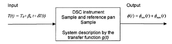
Figure 1 - Schematic representation of a DSC.

The technique is based on a thorough analysis of the response of a DSC (including the apparatus and the sample) toward a stochastically modulated underlying temperature program. Figure 1 is a block diagram of how the TOPEM technique processes the inputs from the DSC into the more understandable outputs of reversing and nonreversing heat flow.

With TOPEM, the input signal is a superposition of an underlying temperature ramp T₀ + β_{u t}(where T₀ denotes the start temperature, β_u is the underlying heating rate, and t is time) and a stochastic temperature modulation δT_(t). The measured heat flow consists of a reversing and a nonreversing component—φ_rev(t) and φ_non(t), respectively. The system (i.e., the instrument including the sample and the pans) is described by the transfer function g(t).

The analysis of the DSC system is based on the following assumptions:

1. The DSC is considered as a linear, time invariant system during a sufficiently long time interval and for a reasonably small temperature modulation.
2. The sample response to the temperature program can be separated into a linear response (reversing heat flow) and a nonlinear response (nonreversing heat flow). It is assumed that the nonreversing processes are slow. This assumption corresponds to an assumption regarding the sample: It is only allowed to exhibit slow nonreversing effects. An effect will be considered slow if its time scale is larger than what has been called a sufficiently long time interval.

These assumptions are the same for all known TMDSC techniques.

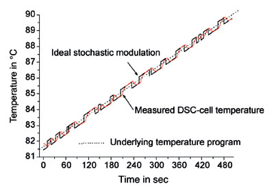
Figure 2 - TOPEM temperature program and measured DSC cell temperature.

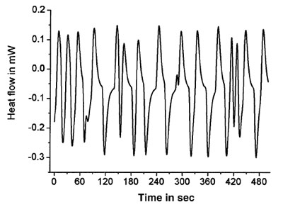
Figure 3 - TOPEM heat flow.

To probe the response of the DSC system, TOPEM makes use of a stochastic temperature modulation. Ideally, the modulation consists of step-like temperature increments and decrements with random interval lengths along the underlying heating rate. The actual DSC cell temperature (see Figure 2) as well as the resulting heat flow (Figure 3) are recorded.

Signal analysis

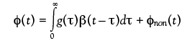
In the absence of nonreversing phenomena and assuming time invariant linear behavior, a DSC system is completely characterized by its transfer function g(t). Thus, the output heat flow φ(t) is related to the input temperature program T(t) according to:

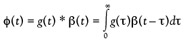
Here, β(t) denotes the heating rate, i.e.,

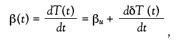
β_υ being the underlying heating rate.

Physically, the transfer function corresponds to the response of the system toward a step-like temperature change at its entry. Due to the assumed time invariance of the system, the integral of the transfer function is equivalent to the specific heat capacity of the sample.

In reality, the temperature and heat flow signals are sampled at a certain rate. Furthermore, time invariance of the system is only valid within a limited time interval and the assumption of linear response is violated if nonreversing thermal effects occur.

Neglecting, first of all, nonreversing processes, the technical problem requires the determination of g(t) (0 ≤ t < ∞) from discrete data in a sufficiently long time frame in which the assumption of time invariance is at least a good approximation. A standard technique to solve this problem is the use of a discrete Laplace transformation (referred to as z-transformation). Thus, the z-transformed Eq. (1) reads as:

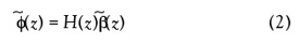
where (z), H(z), and (z) denote the z-transforms of ϕ(t), g(t), and β(t), respectively.

A convenient way to describe H(z) is by setting 

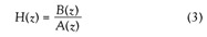
where B(z) and A(z) are polynomials of degree q and p, respectively. Inserting Eq. (3) into Eq. (2), applying the inverse z-transformation and taking into account the discrete nature of the recorded data lead to: 

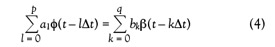
where Δt corresponds to the sampling time interval and a₁ and b_k denote the unknown coefficients of the polynomials A(z) and B(z). Making use of the time invariance of the system in a sufficiently long time interval, this equation can be numerically solved by a least-squares fitting procedure in the considered time interval.

In the presence of nonreversing phenomena, Eq. (1) has to be modified as follows: 

Here, φ_non(t) is the nonreversing heat flow, which describes the nontime invariant heat flow contribution. Applying again the mathematical procedure outlined above, one finds:

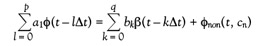
where φ_non(t, c_n) is the nonreversing heat flow that is described by an appropriate expression containing parameters c₀, c₁, . . ., c_n. Again, this equation is solved numerically in a suitable time interval. As a result, the nonreversing heat flow, as well as a parametric description of the transfer function g(t) (coefficients a₁and b_k), are available.

As already noted, integration of the transfer function delivers the quasi-static heat capacity, c_p,₀, of the sample, i.e.,

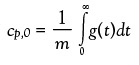
Here, m denotes the sample mass. The quasi-static heat capacity corresponds to the frequency-independent heat capacity that could also be determined using conventional DSC techniques (e.g., the sapphire method) if no excess heat-producing thermal effects occur.

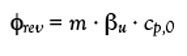
Multiplying the quasi-static heat capacity by the sample mass and the underlying heating rate delivers the quasi-static reversing heat flow, φ_rev(t), i.e.,

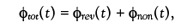
Adding the reversing and nonreversing heat flow yields the total heat flow:

which corresponds to the result of a conventional DSC measurement run at the underlying heating rate. In contrast to other TMDSC techniques, TOPEM offers a simple consistency check. In fact, the moving average of the TOPEM DSC signal in the time interval used for the TOPEM signal analysis is in agreement with the total heat flow as calculated from the reversing and nonreversing heat flow.

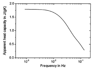
Figure 4 - Frequency dependency of the apparent heat capacity of a sample in thermal equilibrium.

If the transfer function g(t) is known, the response of the system can be calculated for any temperature program, in particular, for a sinusoidal modulation on an underlying temperature ramp. Thus, the well-known frequency-dependent complex heat capacity (including c_p^*, c_p^′, c_p^′′, and the phase angle) can be determined from one single TOPEM experiment in a wide frequency range. This is illustrated in Figure 4, which shows the apparent heat capacity as a function of the applied frequency for a sample in thermal equilibrium.

In thermal equilibrium, the specific heat capacity is frequency independent and corresponds to the quasi-static heat capacity, c_p,₀. The decrease in the apparent heat capacity with higher frequencies (see Figure 4) is therefore due to the limited heat transfer capability of the system. During relaxation phenomena such as glass transitions, for example, the heat capacity becomes a frequency-dependent property of the sample. In such a case, the measured frequency dependency of the heat capacity has to be corrected for the frequency dependency due to instrumental effects. This can be done using the time-dependent quasi-static heat capacity.

In comparison to other TMDSC techniques, TOPEM thus offers the following advantages:

•  A quasi-static heat capacity and quasi-static reversing and nonreversing heat flows are available
• The frequency dependency of the complex heat capacity (c_p^*, c_p^′, c_p^′′, and phase angle) is determined from one single experiment
• The frequency-dependent complex heat capacity can be calibrated using the quasi-static quantities.

TOPEM therefore is an effective tool for heat capacity measurements (quasi-static and frequency dependent) as well as for the separation of the heat flow into a reversing and nonreversing component. Applications for the technique are discussed in Ref. 2.

Conclusion

TOPEM, a powerful temperature-modulated DSC technique, makes use of a stochastic modulation of an underlying conventional temperature program. With the technique, the DSC system is characterized by a parametric model of its transfer function. Based on the transfer function, the quasi-static heat capacity as well as the frequency-dependent complex heat capacity (c_p^*, c_p^′, c_p^′′, and phase angle) are calculated in a large frequency range. In addition, the method provides the quasistatic reversing and nonreversing heat flows. All of this information is available from one single experiment.

References

1. Kraftmakher, Y. Modulation Calorimetry; Springer: New York, NY, 2004.
2. Schawe, J.E.K.; Hütter, T. TOPEM^®: The Latest Innovation in Temperature Modulated DSC. NATAS 34th Annual Conference, 2005.

Dr. Schubnell is a Physicist, Mr. Hütter is an Engineer specializing in the construction of DSC cells, and Dr. Schawe is Polymer Physicist, Mettler Toledo GmbH, Sonnenbergstrasse 74, CH-8603 Schwerzenbach, Switzerland; tel.: +1 806 73 50; fax: +1 806 77 11; e-mail: [email protected]. Dr. Sauerbrunn is the Technical Manager, Mettler Toledo Thermal Analysis, Columbus, OH. Prof. Heitz is a Professor of Mathematics specializing in data extraction techniques, Zürich University of Applied Sciences, Winterthur, Switzerland.