In the three previous columns, we discussed the limit of detection amount LDA, the minimum consistently detectable amount MCDA, and the limit of quantitation amount LQA. In this column we’ll look at an unusual way of describing calibration relationships that makes it possible to visually compare any one of these quantities among multiple measurement methods, even among methods that have different units of measurement.
Figure 1 plots peak area y, measured as milliabsorbance units times seconds (mAU·s), against the amount of analyte x, measured in micrograms (μg), for two different chromatographic methods. The dots in the figure represent raw data; the straight lines give the best least-squares fit and may be considered to be the calibration relationships. Method B is shown in blue and has a sensitivity (the slope of the calibration relationship) of 1.00 mAU·s·μg-1. Method R is shown in red and has a sensitivity of 0.50 mAU·s·μg-1. In a previous column, it was stated that “steeper calibration relationships (more sensitive measurement methods) are usually desirable because they lead to lower values of LDA, MCDA, and LQA,” so it looks like method B is the better method.
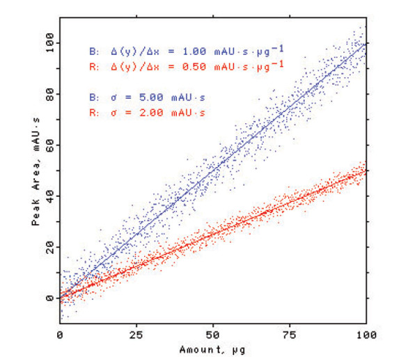 Figure 1 – Raw data and calibration relationships for two chromatographic methods B and R. See text for discussion.
The caveat in the quoted statement is the word “usually.” The statement assumes that the standard deviations of the calibration relationships are equal. But in the example shown in Figure 1, method B has a standard deviation of 5.00 mAU·s, and method R has a standard deviation of 2.00 mAU·s. Clearly these two methods don’t have the same standard deviations.
It is helpful to understand that statisticians often use the standard deviation σ as their unit of measurement. Further, units of measurement have their equivalents: just as 1 gal = 4 qt, 1 σ might equal 5.00 mAU·s.
As a background example, we see the use of the standard deviation as a unit of measurement in the equation for the symmetrical two-sided confidence interval for the true mean μ based on a single measurement y and a known standard deviation σ: μ = y ± zσ, where σ can be interpreted as a (statistician’s) unit of distance along the y-axis and z is simply a value taken from a statistical table that tells us how many of the statistician’s units we have to go on either side of y to include μ with a given level of confidence.
Knowing that statisticians like to measure in units of the standard deviation, John Mandel made the useful suggestion that responses could be measured in units of their standard deviations.1Figure 2 shows the transformed chromatographic responses from Figure 1. Note that the units of raw response and the units of their standard deviation are the same (e.g., mAU·s), so dividing a response by its standard deviation gives a unitless number (the Mandel response) that represents the number of standard deviations of that response in that response. The slopes of the calibration relationships are thus expressed in units of μg-1. In Figure 2, the slopes of the transformed calibration relationships are 0.20 μg-1 for method B, and 0.25 μg-1 for method R. Now method R appears to be the better method (steeper calibration relationship), and it is.
 Figure 2 – Mandel responses and calibration relationships for two chromatographic methods. See text for discussion.
Using the MCDA as an example, if the MCDA is taken to be the amount of analyte that gives a signal 6.6 standard deviations above the mean of the blank, then Figure 3 shows the amounts of analyte required to provide this signal strength: 33.0 μg for method B and only 26.4 μg for the better method R.
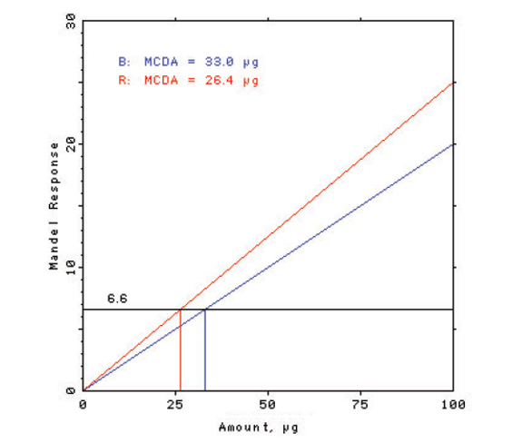 Figure 3 – Visual comparison of
 MCDA
for two chromatographic methods. See text for discussion.Because the Mandel response is unitless, similar plots can be made for groups of measurement methods that have unrelated measurement units. For example, mass spectrometry with units of ion·s, chromatography with units of mAU·s, and cyclic voltammetry with units of μA (for ipc, say) can be compared. In the hypothetical simulation shown in Figure 4, mass spectrometry is seen to have the lowest MCDA.
 Figure 4 – Visual comparison of
 MCDA
for three measurement methods that have unrelated units of measurement for their raw responses. See text for discussion.Similar plots can be made for LDA and LQA, with (say) Mandel responses of 3.3 and 10.0. This ends the series of columns on limits of detection and related concepts. In the next column, we’ll consider the effect of the resolution (or “graininess”) of raw data on statistical calculations.
Reference
- Mandel, J. The Statistical Analysis of Experimental Data; Wiley: New York, NY, 1964.
Stanley N. Deming, Ph.D., is an analytical chemist masquerading as a statistician at Statistical Designs, El Paso, Texas, U.S.A.; e-mail: [email protected]; www. statisticaldesigns.com