In the two previous columns, we discussed the limit of detection LD, the minimum signal strength above which we can state with at least a given level of confidence (e.g., ≥99.95%) that analyte is present; and the minimum consistently detectable amount MCDA, the smallest amount of analyte that can be detected with at least a given level of confidence (e.g., ≥99.95%). Setting the LD requires specifying the false positive risk α (e.g., ≤0.0005) of detecting analyte when, in fact, it is absent; setting the MCDA requires specifying the false negative risk β (e.g., ≤0.0005) of stating that analyte is not detected when, in fact, it is present. The two risks are set in consultation with the client. In general, the two risks will not be equal.
In this column, we discuss the limit of quantitation LQ and the corresponding limit of quantitation amount LQA. The limit of quantitation often has less to do with statistics than it has to do with ego.
To get started, look at Figure 1. Assume a sample has been prepared that contains the limit of detection amount LDA of analyte. On the average, this will give a signal equal to the limit of detection LD. In Figure 1, eight representative measured values for the LDA are shown near the signal axis as black squares enclosed by a Gaussian curve with a standard deviation σb, the standard deviation of the blank. All eight data points should appear above the LDA, but have been shifted to the left and are spread out for clarity. When each of these measured signals is converted to an amount through the calibration relationship, the resulting data points on the horizontal amount axis are contained within their own Gaussian curve with a standard deviation we’ll call σa.
 Figure 1 – The relationship between the standard deviation of the signal
 σ
b, the standard deviation of the analyte σ
a, and the sensitivity of the measurement method (i.e., the slope of the calibration relationship).Following the definition given by the International Union of Pure and Applied Chemistry (IUPAC), the sensitivity of a measurement method is the slope of the calibration relationship1 (not the smallest amount of analyte that can be detected). Here’s an important fact (see Figure 1):
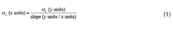
Thus, for a given uncertainty in the measured signal (σb), a calibration relationship with a larger slope (a more sensitive measurement method) gives a smaller standard deviation σa on the amount axis (see the redcircled inset in Figure 1). As we’ll see in the next column, steeper calibration relationships (more sensitive measurement methods) are usually desirable because they lead to lower values of LDA, MCDA, and LQA.
Before we leave Figure 1, let’s assume we’ve used α = 0.0005 and we’ve set LD at μb + 3.3×σb. Working through the calibration relationship, a bit of geometry shows that, if LD is 3.3×σb above μb, then LDA must be 3.3×σa to the right of zero on the horizontal axis, that is, LDA = 3.3×σa, and the standard deviation on the amount axis at LDA is σa. Hold that thought.
Many analysts (bioassayists, especially) are obsessed with the percent relative standard deviation %RSD, sometimes called the percent coefficient of variation %CV, defined as:
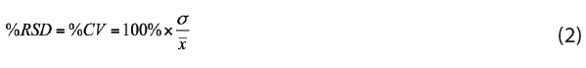
where x̄ is strictly the mean of several measurements, usually the reportable value. So, what is the %RSD at the LDA? Plug and chug:
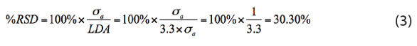
Thus, for our teaching example (α = 0.0005, LD = μb + 3.3×σb), the percent relative standard deviation at the limit of detection amount is about 30%.
When I was an undergraduate student at Carleton College, Professor Richard W. Ramette taught us the importance of precise work—Class A glassware, the “double-dozen” technique for diluting in a volumetric flask, etc. We would have been ashamed to turn in a lab report with a %RSD of 30%! Is that a quantitative result? He wouldn’t think so. It’s a pretty “fuzzy” result, at best. There’s too much uncertainty in that number to be considered quantitative!
But at the LDA, that’s the best we can do. It is what it is, almost by definition (and because of our specification of α = 0.0005).
So, what about the MCDA? Are things more quantitative there? If α = 0.0005 and β = 0.0005, then MCDA = 2×LDA = 6.6×σa, which gives:
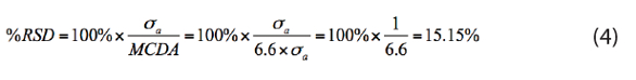
Although Ramette and his students would probably not consider this to be a quantitative result, in my experience and opinion, the bioassay community seems to accept 15 %RSD as a “pretty good” quantitative result, not because of anything having to do with “fitness for use,” but rather because it’s about the best they can do given the small volumes they have to work with.
Again, I have great respect for bioassayists. I will simply note that a relative standard deviation of 15% is a large uncertainty if you’re trying to show that a product is within 80% to 125% of the label claim. Such a large relative standard deviation in the raw data usually requires expensive replicate measurements to reduce the uncertainty of the reportable mean. But that’s another column.
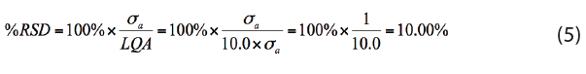
So … what’s a quantitative result? Just like setting the α and β risks, deciding how small the %RSD must be for a result to be considered “quantitative” requires discussions between the analyst and client. If, for example, it is decided that the %RSD must be no more than 10%, then the LQA must be 10.0×σa:
The three “benchmarks” in our discussion of LDA, MCDA, and LQA are shown in Figure 2. On the horizontal amount axis, values at or above the LDA are said to be confidently detected; values at or above the MCDA will be consistently detectable; values at or above the LQA are said to be quantitated. An example of the application of these ideas to trace organic analysis has been given by Locanto.2
 Figure 2 – Interpretation of
 LDA
, MCDA
, and LQA
discussed in this column. The width of each colored rectangle is equal to σ
a.If q is the amount of analyte measured in units of σa (e.g., q = 6.6 for MCDA), the relationship between q and the %RSD is shown in Figure 3. The values of q for the LDA and MCDA are set by α and β, respectively; the value of q for the LQA is set by the analyst and client and their agreement on how low the %RSD must be for the measurement to be considered “quantitative.”
 Figure 3 – The relationship between the amount of analyte measured in multiples of
 σ
a (q
) and the %RSD. Specific values are shown for LDA
, MCDA
, and LQA
as discussed in this column.In the next column, we’ll look at an interesting way of constructing calibration relationships so that various disparate methods of measurement can be compared quickly in terms of their relative values for LDA, MCDA, and LQA.
References
- https://goldbook.iupac.org/html/S/S05606.html
- Loconto, P.R. Use of weighted least squares and confidence band calibration statistics to find reliable instrument detection limits for trace organic chemical analysis. Am. Lab. 2015, 47(7), 34–9.
Stanley N. Deming, Ph.D., is an analytical chemist masquerading as a statistician at Statistical Designs, El Paso, Texas, U.S.A.; e-mail: [email protected]; www.statisticaldesigns.com