The previous installment (Part 38, American Laboratory, May 2010) outlined the regression-diagnostic steps needed when replicates are not exact. This article will illustrate the protocol using the nitrite data that have been used throughout this series (please refer to Part 38 for details on each step). To avoid an “overload” of plots and numbers, only the results for the middle concentration (62.5 ppt) will be illustrated for Steps 1 and 3.
Step 1: Check responses for trends within each group of concentrations
Inspection for trends showed none. For 62.5 ppt, the plot and p-value (for the line’s slope) are shown in Figure 1.
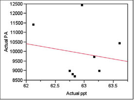
Figure 1 - For the target concentration of 62.5 ppt, a plot of peak area (PA) vs concentration (ppt). A straight line has been fitted using ordinary least squares. The p-value for the line’s slope is 0.6926, meaning that there is no trend to the data.
Table 1 - Listing of target concentrations and the means of the actual concentrations achieved
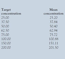
Step 2: Calculate the mean concentration for each target-concentration group
The mean values are shown in Table 1.
Step 3: Scale the actual responses to each mean
When this step is performed, the slope of the line is 83.50, which is the dy value needed to scale the actual peak areas (PAs) to each concentration’s mean. In Figure 2, the scaled PAs for the 62.5-ppt target concentration all plot at the mean concentration (62.94 ppt). Each raw-data point and its corresponding scaled value have the same marker shape/color.
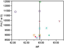
Figure 2 - In this diagram, each original data point has the same shape/color as its corresponding scaled value. “T” stands for true (or actual) PA and “S” stands for scaled PA. All “S” values fall on the mean-concentration line.
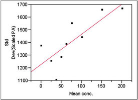
Figure 3 - Plot used to model standard deviation. The slope’s p-value (0.0088) is significant, meaning weighted least squares is needed as the fitting technique.
Step 4: Model the standard deviation
The results of the standard deviation modeling are shown in Figure 3. The p-value for the slope is 0.0088, meaning that the slope is statistically significant. (See Part 8, American Laboratory, Nov 2003, for a discussion of the fundamentals of this type of modeling and calculation of weights.) Thus, weighted least squares (WLS) is needed for the fitting technique.
When Step 3 is repeated, using WLS to fit the line, the slope is 83.56. When ordinary least squares (OLS) was used originally, the slope was 83.50. This difference results in an insignificant change in the scaled responses and can be ignored.
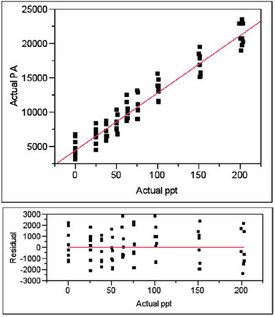
Figure 4 - Plot of actual PA vs actual concentration, regressed with a straight line using weighted least squares. Also shown is the residual pattern.
Step 5: Test the proposed model for the actual data
Figure 4 shows the plot of the actual PAs versus the actual concentrations; the proposed model is a straight line and WLS fitting (using the weight from Step 4) is used. The residual pattern is also shown; the distribution of points appears to be random about the zero line. A lack-of-fit (LOF) test will allow a formal decision on the adequacy of the model.
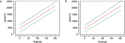
Figure 5 - Calibration curves with prediction intervals (at 95% confidence) for: a) actual PA vs target concentration and b) actual PA vs actual concentration.
Step 6: Perform an LOF test, using the scaled responses and mean concentrations
The p-value for this test is 0.8246, supporting the conclusion (in Step 5) that a straight line is an adequate model.
In Part 12 (American Laboratory, Jul 2004), the slope was found to be insignificant, but only barely so; the actual p-value was 0.0109. Figure 5 shows the plots (with prediction intervals) for the two regressions. The differences are only slight.
Mr. Coleman is an Applied Statistician, Alcoa Technical Center, MST-C, 100 Technical Dr., Alcoa Center, PA 15069, U.S.A.; e-mail: [email protected]. Ms. Vanatta is an Analytical Chemist, Air Liquide-Balazs™ Analytical Services, 13546 N. Central Expressway, Dallas, TX 75243-1108, U.S.A.; tel.: 972-995-7541; fax: 972-995-3204; e-mail: [email protected].