In an attempt to demystify artificial neural
networks (ANNs) and to set the
tone of this paper, it is best to start by
saying that ANNs are mathematical functions
of the form y = f(x, w), where y is
the output or response that is determined
from a given input x by a series of calculations
through a network of connected
processing elements or nodes. This article
demonstrates the feasibility of utilizing a
Microsoft® Excel™ workbook for defining,
training, and subsequently using ANNs as
a prediction tool. The example given here
involves the prediction of nitrogen oxide
(NOx) emissions from boilers. It is very
important to be able to predict the emissions
of pollutants such as CO and NOx
in boilers in order to determine the effectiveness
of the combustion process and to
evaluate the environmental contribution
of gas emissions. This requires measured
data such as effluent temperature and gas
flow rate.
The nodes or neurons are arranged in
layers and are connected by unidirectional
communication arcs, which carry
numerical data. The input nodes represent
a set of variables, x, and the output
nodes correspond to the predicted output
set of y variables. These two sets of
nodes form the input and output layers,
respectively. The information between
layers is processed through various intermediate
layers, the so-called hidden
layers. The parameters that modify the
information transferred from one layer
to the next, w, represent the strength of
the connection between the nodes, and
whose numeric values give the network
its predictive power.
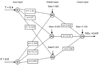
Figure 1 - Schematics of a three-layer neural network model.
The neural network in Figure 1 contains
three layers. The input layer has two nodes,
I1 and I2, one for T (temperature) and one
for F (flow), respectively. The hidden layer
has three nodes, H1, H2, and H3; the output
layer has only one node, O1, which
corresponds to the calculated concentration
of NOx.
Calculations in the ANN start
when values are applied to the
input nodes. These inputs are then
multiplied by the weights wk,i connected
to all nodes in the hidden
layer. The products are summed
up for each node and a bias is subtracted
(sum = Σxkwk,i – bk). xThis
sum is passed along to an activation
function to produce the output
of the node; the sigmoidal
function is the most commonly
used activation function, f(sum) =
1/(1+exp(-sum)). The resulting values
are then used as the inputs to
the output layer. Each neuron in
the output layer receives weighted
inputs minus bias from each neuron in the
hidden layer to determine the activation
function of the output layer, which corresponds
to the neural network output.
The activation function serves to model
nonlinear behaviors. The input nodes act
as distribution nodes, with no calculations
associated; the inputs are just transferred
to the nodes in the hidden layer.
For example, in the neural network model
of Figure 1, operations are performed in the
hidden nodes that receive the two inputs
(input #1 has a value of 0.4 and input #2 a
value of 0.6). Each input has a corresponding
weight that connects to the hidden
nodes (weight #1 connects input #1 and
has a value of –1.26, etc.). Three values
of f(sum) will be calculated, one for each
node in the hidden layer 0.341, 0.979, and
0.947, respectively. Then, the weighted
sum of inputs and calculation of the activation
function for the output node are
applied, and a value of 0.609 is obtained
in the network output.

This particular method of performing the
calculations in the ANN is associated with a
structural design named feed forward. If the
actual value of the target is equal to 0.62, the
error between the target value and the output
would be equal to –0.011 (i.e., 0.62 – 0.609 = –0.011). All errors for all the observations in
the dataset are calculated for these particular
sets of weights and bias values.
When a neural network is trained, the
weights and bias terms of neurons are
adjusted individually. Training a neural
network is an iterative process; it uses a
nonlinear optimization algorithm to obtain
the optimal values of the weights. The data
must be divided into two subsets: a training
dataset and a test dataset. An error back-propagation
is the most widely used algorithm,
and it is known as a learning algorithm.
A full mathematical explanation of
this algorithm can be found elsewhere.1–3
Initially, the connection weights and bias
are set to random values. The weights are
then adjusted until a training error criterion
is minimized, that is, until learning is
successful. The most common convergence
criterion is the mean squared error (MSE),
which is the squared difference between
the actual output and the predicted output,
divided by the number of observations
(patterns) of the training dataset.
Neural networks were studied as early as
the 1940s by McCulloh and Pitts.4 However,
they did not become popular until
around 1985, when the method of back-propagation
for training neural networks
was introduced by Rumelhart et al.5 Neural models are now enjoying a resurgence, and
there is a substantial amount of research
in the area of neural networks, because of
their ability to represent nonlinear relationships,
which is useful in making function
approximation, forecasting, and recognizing
patterns.6,7
Use of Excel to train a neural network
The objective of this study was to develop
a simple, easily understood methodology
for training neural networks using an Excel
workbook. Data from a boiler stack were
used to build and train a neural network
that predicts the concentration of NOx
emissions. A combustion analyzer was used
to measure NOx in the flue gas.
The Excel workbook that predicts the
NOx emissions consists of three modules
(DATA, TRAINER, and QUERY). The
DATA worksheet is an interface for users
to keyboard the data and normalize them.
The TRAINER worksheet is an interactive
interface and work area. The user
can interact with the spreadsheet by setting
and adjusting parameters needed for
training the neural network. The QUERY
worksheet is designed for query and computing
results.
Configuring the DATA worksheet
The data must be preprocessed in order for
the ANN to effectively learn from them.
All values that appear to be scattered
far away from the majority of values are
considered outliers and must be excluded
from the dataset. The numeric data of all
the variables are linearly scaled between
0 and 1, considering the minimum and
maximum values. This scaling of variable
values is made in order to avoid using
data spanning different orders of magnitude.
Following the common practice,
the dataset to train the network was made
by randomly selecting about 70% of the
database. The remaining 30% of data
were then used to check the generalization
capability of the model.
Microsoft Excel makes it possible to
access more than one worksheet. Each
worksheet is represented in the bottom
section of the interface with a tab. The
left-most tab is marked Sheet1. The
second from the left is marked Sheet2.
The last is marked Sheet3. To rename a worksheet, the user double-clicks its
sheet tab and then types a new name.
Once this is done, the user changes
the tabs Sheet1, Sheet2, and Sheet3
to the new names DATA, TRAINER,
and QUERY, respectively. To move
between the different worksheets, the
corresponding tabs are clicked.
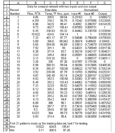
Figure 2 - DATA worksheet.
The steps below are followed:
- Enter the number for each record
into column A, type 1 into cell
A4, and the equation =A4+1 into
cell A5. Then highlight cell A5;
the cursor box will enclose the
cell, and a small black square will
be seen at the lower right corner
called the fill handle. Point to the
square (the pointer should change
to a thin cross), press and hold the
left mouse button, drag the pointer
downward to cell A33, and release.
This yields a column of serial numbers
by copying the equation from
cell A5 down to and including A33.
See Figure 2.
- Enter the headings for columns B, C,
and D into rows 2 and 3.
- Enter the values for the flow, temperature,
and NOx into columns B, C, and
D, respectively. These will correspond
with the actual values for input nodes
1 and 2 and the output node of the
network.
- Enter the function to determine the
largest number for each input and output
node, starting in cell B36 to cell
D36, using the MAX function. To do
so, position on cell B36 and click on
the Insert Function button to the left
of the formula bar. Several functions
are available; select MAX and the
functions arguments dialog box will
pop up. With the mouse, select range
B4:B33, click the OK button, then
into cell C36 enter MAX(C4:C33);
into cell D36 enter MAX(D4:D33).
- Enter the minimum values for data
values for each input and output node
as in step 4, using the MIN formula,
into cells B37 to D37.
- The next step is to normalize the data
by subtracting the minimum value
and dividing by the difference of the
maximum minus the minimum. The
normalized values for input #1 of column
B will be in column E. Into cell
E4 type (B4-$B$37)/($B$36-$B$37).
Copy this formula into the rest of column
E; use the fill handle to copy values
into neighbor cells from rows 4 to
33, as in step 1. When this is done, cell
references that do not include $ signs
are updated (cell address B4 in the formula
changes to B5, B6, etc.), whereas
cell references with $ signs (cells with
absolute address) are not; a simple way
to do this is to hit the function key F4
when typing the cell address. This is
important because $B$36 and $B$37
are fixed parameters. Do the same for
input #2 values on column F and the
output values on column G using the
proper address for max. and min. Save
the workbook.
This ends the easy part of laying out the
DATA worksheet. The TRAINER worksheet
is prepared as shown below.