In the previous installment (American Laboratory, Oct 2011), the terms that contribute to R2 were defined and a formula relating them was developed. This article will show how R2 is calculated and explain shortcomings associated with this statistic.
A brief review is in order first. The three terms are: 1) sum of squares for the model (SSModel, the amount of variation explained by the model), 2) sum of squares error (SSError, the variation not captured by the model plus the random noise inherent in the data), and 3) total corrected sum of squares (SSTotal). The relationship among the terms is:
SSModel + SSError = SSTotal (1)
The “expanded” version of the formula is:
Σ(ypi – yp-mean)2 + Σ(yi – ypi)2 = Σ(yi – ymean)2, (2)
where:
ypi = a y-value predicted by the proposed model,
yp-mean = the mean of all the ypi values,
yi = an actual y-value (or response),
ymean = the mean of all the actual y-values (i.e., the “grand mean”).
Lastly, the definition of R2 is the proportion (of the variation) that can be explained by the regression that has been performed. Typically, the statistic is stated as a percentage, in decimal form.
How does the above definition translate into a formula for R2? Since SSModel is the amount of uncertainty captured by the model and SSTotal is the total variation, the proportion is simply:
R2 = SSModel/SSTotal (3)
Another form of this expression can be obtained if Eq. (1) is first rearranged to give:
SSModel = SSTotal – SSError (4)
Substituting Eq. (4) into Eq. (3) gives:
R2 = (SSTotal – SSError)/SSTotal (5)
or:
R2 = (SSTotal/SSTotal) – (SSError/SSTotal), (6),
which simplifies to:
R2 = 1 – (SSError/SSTotal) (7)
Since (SSError/SSTotal) is the proportion of the variation that is left over (i.e., not “eaten” by the model), R2 can be seen as an indication of how far away the regression is from perfection (i.e., from R2 = 1). In other words, a higher (SSError/SSTotal) will result in a lower R2.
Why is this statistic insufficient for evaluating the adequacy of a chosen model? The answer lies in the definition of SSError (see review paragraph above), which is simply a sum of its two components. R2 cannot reveal how much of the error is from random noise. If the noise is very large, then the presence of an acceptable model can be masked.
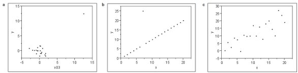
Figure 1 - Scatterplots for three different data sets: a) leverage point, b) outlier, c) typical noise. What is the common thread? See text for the answer.
Other traps lie in wait. Consider Figure 1. Plot (a) contains a cluster of data plus one point at a much larger x-value (this last point is called a “leverage point” because it can act as a lever that strongly influences the slope and intercept estimates). Plot (b) appears to be a perfect straight line, with the exception of one outlier. Plot (c) contains data that seem to trend and exhibit random noise (in other words, fairly typical noisy calibration or recovery data). Now for a pop quiz. What is the common thread among the three? The answer is as follows. If a straight line is fitted to each of the data sets, using ordinary least squares as the fitting technique, then the value of R2 is almost identical for all three cases (0.670, 0.644, and 0.670, respectively)! The statistic has no ability at all to discriminate among different reasons for deviation from perfection.
A second trap exists when the urge to try higher-order polynomials creeps into the regression landscape. For any data set, adding the next-higher x-term will always increase the R2 or leave it unchanged (when compared with the previous, lower-order model). The reason is that every additional term contributes an additional coefficient, which can be tweaked along with all the coefficients from the preceding model.
A key objective of regression is to have the curve go through the mean of the responses at each x-value. Thus, as more coefficients become available, there is greater opportunity to “fine-tune” in pursuit of this goal. However, the price of such an outcome is that the overall shape of the fitted model may be quite odd and implausible; the resulting meandering is not likely to be intrinsic to the actual data.
This trap is more severe than simply overfitting by going to higher and higher polynomials. As will be seen below, adding any term to an existing model will raise R2 (or leave it unchanged).
Consider the following (simulated) challenge given to fictitious Laboratory XYZ. They have been asked to perform an analytical test that has several quality requirements. One mandate is to generate a calibration curve with a “high value for R2.” Another directive is to analyze five replicates of each of six different standards.
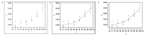
Figure 2 - The scatterplot for a simulated data set, as well as the fitting of two different models (each time using ordinary-least squares): a) scatterplot of data, b) quartic model; R2 = 0.88380, c) quadratic model plus a phases-of-the-moon term; R2 = 0.88372. See text for details.
The laboratory’s chemists set out on their mission and generate the required data. The scatterplot is shown in Figure 2a. Standard-deviation modeling shows that ordinary least squares is the appropriate fitting technique. Since the data exhibit curvature, the analysts begin by fitting a quadratic; R2 = 0.88226. In an attempt to raise this value, they try a cubic, but gain very little (R2 = 0.88234). Undeterred, the scientists press on to a quartic, which gives a more significant increase (R2 = 0.88380).
About this time, a colleague comes by to see how the regression work is going. Upon hearing that the fitting is up to a fourth-order polynomial, the co-worker suggests adding the phases of the moon to the quadratic, as an alternative to cubic or quartic. Application of this advice gives an R2 of 0.88372, which competes nicely with the quartic! In fact, the two curves are almost identical (see Figure 2b and c).
What on earth (or moon, perhaps) is going on?!? The similarity of Figure 2b and c is purely a coincidence of this simulation (and was not planned by the authors!), but the rise in R2 values with the addition of the “odd” term is not coincidental. Indeed, even something as unrelated to analytical data as the phases of the moon will never decrease (and will generally increase) the R2 of the previously fit and simpler model, which in this case is a quadratic.
By now, the reader may be wondering what to do, especially since R2 is so widely used within the analytical community. A more realistic version (R2adjusted, usually abbreviated as R2adj) exists and will be discussed in the next installment. Also included will be a review of a robust approach to diagnosing regression models. Please stay tuned!
Mr. Coleman is an Applied Statistician, and Ms. Vanatta is an Analytical Chemist, e-mail: [email protected].