Statistics in the Laboratory: Significant Digits and the Granularity of Data

A true story: one of my former graduate students called me and said, in effect,

“Help. I know I’m a good analytical chemist, but my company is making me look like a perfect analytical chemist.”

“What’s your company doing?” I asked.

“My company has a policy that says all numbers have to be rounded to no more than four significant digits, and my numbers are 99.967, 99.973, and 99.969 with a mean of 99.96967 and a standard deviation of 0.003055. I’m precise, but not perfect.”

“So?”

“So, my company says I have to round my numbers to 99.97, 99.97, and 99.97 with a mean of 99.97 and a standard deviation of zero! I’m good, but not that good.”

“Ah!” I said. “You’re clearly the beneficiary of an ill-conceived company policy.”

I then referred her to the classic 1951 text by Walter J. (“Jack”) Youden, Statistical Methods for Chemists¹ :

… to determine the precision of the measurements, it is necessary to retain in the data the terminal decimal places which are often dropped. It is a generally followed practice not to give more decimal places than will be meaningful in any use made of the results. This often leads investigators to round off the data and thus suppress a large part of the information originally available for determining the precision. The extra decimal places that are of no consequence to the user are obviously just the ones that do contain the information on the variation between determinations. These extra decimal places should be reported so that the precision may be determined.

As Youden suggests, too many digits to the right won’t hurt your statistical calculations, but too few digits to the right will hurt your statistical calculations. Policies that limit the number of digits that can be reported often interfere with meaningful statistical calculations.

I have come to loathe the concept of “significant digits.” If I’m going to limit the number of digits reported, I do it only at the very end of a series of calculations, and then only after consultation with the client so everyone understands what the final number means … and what the final number doesn’t mean. For example, even if the rules of significant digits have been followed, it is folly to assume (as is often done) that the uncertainty in the result is only one unit in the final digit.

To avoid suffering from significant digits, my preference is to attach a statistical confidence interval to the reported result (e.g., “there’s a 95% chance that the interval from 99.92 to 100.02 contains the true result”). A confidence interval is statistically meaningful, and it can be used to convey a visual interpretation of the uncertainty in the result.

Moving on to a related issue, my student’s experience points to the broader (but rarely discussed) concept of “graininess” or “granularity” of the data—that is, the resolution of the data. It is a quantal concept. I take the graininess (or granularity) to be the number of units of the last reported digit that fit into the range of the data. In my student’s extreme example above, the graininess of the original data was the number of times 0.001 goes into the difference 99.973 – 99.967 = 0.006, a graininess of 0.006/0.001 = 6 (often expressed as “one part in six”). However, after applying the company’s rule, the graininess of the data becomes the number of times 0.01 goes into the difference 99.73 – 99.73 = 0.00, a graininess of 0.00/0.01 = 0! Youden’s valid concern, then, is that statistics become distorted when the graininess gets too low.

With modern instrumentation, raw data values are often multiplied by calibration factors or other constants with the result that reported values might appear to have a greater graininess than they actually possess. Table 1 gives six measured results with an apparent graininess of (110.366 – 108.381)/0.001 = 1985. However, pairwise subtractions between data points reveals a consistent difference of 0.397, the smallest “unit” of change. Thus, the true graininess of the data in Table 2 is (110.366 – 108.381)/0.397 = 5. When I begin to work with an unfamiliar data set, I will often sort a data set in increasing order, take pairwise differences, take pairwise differences of differences, etc. If I find zeros beginning to appear down this chain of repetitive differences, I strongly suspect that “multiplicative distortion” exists in the apparent graininess of the data set.

Table 1 – An example of apparently large graininess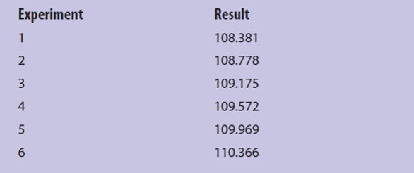

Table 2– Data from Tattersfield and Gimingham²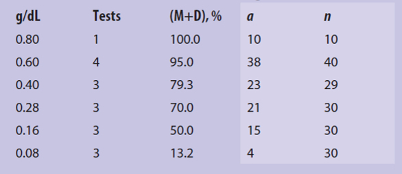

Sometimes the data are inherently grainy: additional digits to the right just can’t exist. An example occurs in animal bioassays where, for humane reasons, the protocol limits the number of animals used.³ In vaccine testing, for example, the group size at each of only four doses might be 10 animals. This corresponds to a graininess of 10 for the response at that dose. When the fraction f of animals affected is calculated, only eleven fractions are possible at each dose: f = [0, 0.1, 0.2 … 0.9, 1].

The curve in the top panel of Figure 1 shows an underlying logit relationship between the fraction of animals affected and the log₁₀(dose, g/L). Expected experimental results are shown as blue dots. The expected fractions for log values of –9, –8, –7, and –6 are 0.1, 0.3, 0.7, and 0.9, respectively. Unfortunately, animals don’t always behave as expected, and results similar to those shown in the bottom panel of Figure 1 are often obtained. Here the observed fractions are 0.1, 0.3, 0.8, and 0.7, with the two unexpected results shown as red dots. The two highest doses exhibit a phenomenon called either “inversion” or “non-monotonicity”— that is, as the log₁₀(dose, g/L) increases, the last response goes down instead of continuing upward. Inversion is not unusual and happens fairly often with small statistical samples like this (a group size of 10). Unfortunately, not everyone understands the behavior of small statistical samples. Thus, some “assay acceptance criteria” flag inversion as a “fail” and require that the assay be carried out again. Statisticians call this censoring the data, i.e., eliminating unwanted results. I don’t agree with the philosophy of repeating these assays—there’s nothing statistically unusual about inversion.

Figure 1 – Top: the underlying logit relationship between the fraction of animals affected and the log₁₀(dose, g/L), with expected experimental results superimposed as blue dots. Bottom: same as above, but with unexpected experimental results superimposed as red dots.

Interestingly, Nick Brown and James Heathers, the “data thugs,” use a technique called the “granularity-related inconsistency of means, or GRIM,” as a technique for finding mistakes in research papers.⁴ When an average of only a few integer values is taken, not all values are possible in the result. For example, the average of only four integers cannot be reported with the sequence 257 appearing after the decimal point—only 0, 25, 5, and 75 are possible. If a researcher were to report an impossible value for the average of four integers (e.g., 23.257), Brown and Heathers would flag the paper for further scrutiny. (Though not related to graininess, the frequency of leading digits in large data sets is another interesting way to find suspicious data.^5-7)

Although at the time I didn’t know what to call it, I once came across a GRIM example in a 1927 paper by Tattersfield and Gimingham² describing an early structure-activity study that involved the use of fatty acid surfactants as insecticides for Aphis rumicis, a type of aphid. Table 2 shows the effect of decreasing doses of lauric acid (dodecanoic acid) in tests that were each said to contain 10 aphids. The first column gives the dose of lauric acid in g/dL given to the group, and the second column gives the number of tests (with, presumably, 10 aphids per test). The third column gives the percentage of moribund (M, about to die) plus dead (D) aphids in the group. The desired effect is that M+D be large. The last two columns in Table 1 were not given in the original paper.

The percentage of M+D for a dose of 0.40 g/dL looked suspicious. How could a value of 79.3 result from division by 30 (three tests of 10 aphids each)? It can’t. My conclusion was that the total number of aphids (n) was 29, not 30, and that 23 of the aphids (a) were moribund or dead: a/n = 23/29 = 0.793103 ~ 0.793 = 79.3%. (And yes, I did round the result to give the same number of digits as appeared in Tattersfield’s and Gimingham’s paper.) I wonder where the missing aphid went.

To conclude, if you’re going to “do statistics” on data, be aware of the graininess of the data and use caution when interpreting the statistical results if the graininess is low.

Reader responses to the previous column

Howard Mark (The Near Infrared Research Corporation) has correctly criticized the way I lumped mass spectrometry in with other methodologies to illustrate Mandel sensitivity: “In order for Mandel’s method to work, the data must be Normally distributed. That is a reasonable assumption for the other methods, and even for Mass Spec at high ion counts where the Poisson distribution approximates the Normal distribution well. But at low ion counts, where low concentrations mean that it’s likely to be more important to get the details right, the underlying Poisson distribution of the shot noise of the ion counts will make itself felt and potentially lead to incorrect comparisons.”

I agree. In addition to the non-normality of the Poisson distribution at low ion intensities (it is asymmetrical with a long tail on the high side), the standard deviation of the Poisson distribution of ion intensities is not constant but increases as the square root of the ion intensity. Statisticians use the term heteroscedasticity for this “variable variability.” Thus, it is not meaningful to talk about the standard deviation of a mass spectrometric method—there is no one value that applies to all values of response. However, if there were a constant “dark current noise” in the detector that swamped the theoretical Poisson value at low levels of response (and made the noise structure homoscedastic), then the Mandel concept would again apply.

Edward Voigtman (Emeritus, Department of Chemistry, University of Massachusetts Amherst) made a similar point about the homoscedastic requirement for the Mandel concept to work, and also pointed out that the response must be linear in the region of interest: “if it is desired to compare the ‘detection power’ of two methods, it suffices to compare their respective limits of detection, assuming both methods have linear response functions/calibration curves and also assuming both methods have homoscedastic noise that is … Gaussian distributed.”

I thank both readers for their comments, and I will try to be more careful with my examples in the future.

References

1. Youden, W.J. Statistical Methods for Chemists. Wiley: New York, NY, 1951.
2. Tattersfield, F. and Gimingham, C.T. Studies on contact insecticides. Part V. Annals of Applied Biol. 1927, 14, 217.
3. Russell, W.M.S. and Burch, R. L. The Principles of Humane Experimental Technique. Methuen: London, 1959.
4. Marcus, A. and Oransky, I. The data thugs: Nick Brown and James Heathers have had striking success in catalyzing retractions by publicly calling out questionable data. Science 2018, 359(6377), 731.
5. Diaconis, P. The distribution of leading digits and uniform distribution Mod 1. Annals of Probability 1977, 5, 72–81.
6. Diaconis, P. and Freedman, D. On rounding percentages. J. Am. Statistical Assoc. 1979, 74, 359–64.
7. Benford, F. The law of anomalous numbers. Proceedings of the American Philosophical Society 1938, 78, 551–72.

Stanley N. Deming, Ph.D., is an analytical chemist masquerading as a statistician at Statistical Designs, El Paso, Texas, U.S.A.; e-mail: [email protected]; www.statisticaldesigns.com