With many things in life, the quality and usefulness of the outcome depends in large measure on the care with which the event is planned. Calibration is no exception. While a statistical evaluation can be made on any set of calibration data, the results can be meaningless if the design of the study is flawed. This column will discuss the steps that should be taken to develop a calibration study. In addition, some example designs will be presented. It must be stressed, however, that there is no one-formula-fits-all answer. Every calibration situation is different and there is no substitute for careful thinking.
The following four steps will help ensure that a successful calibration study is conducted:
- Decide the objectives of the study
- Propose a model for the calibration curve
- Choose the confidence level for the curve
- Design the study carefully.
The following discussion will look at each step in more detail.
Objectives
First and foremost, one must decide what should be accomplished in the study. In other words, when sample results are predicted from the calibration curve, what topics should be addressed? Topics to consider include:
a) Detection limits (DLs). Will the laboratory be pushing the sensitivity of the instrument so that detection limits are an issue? If so, how low of a detection level is needed? When trace work must be done, as many concentrations as possible should be included in the low region. The study should also include a blank, at least one level that is below the desired DL, and at least one concentration above the desired DL.
b) Data behavior. In the plot of response versus spike concentration, is curvature in the data expected for any of the analytes? (The answer here is usually based on empirical data or physical/chemical principles.) If a nonlinear response is expected (e.g., polynomial), concentrations should be added in the area(s) of changing slope. Otherwise, the wrong calibration model may be selected, and a biased (i.e., consistently incorrect) estimate of the calibration function could result.
c) Precision. What level of precision is needed? This answer depends in part on the consequences of a "wrong" answer. If someone's life depends on the result, the data will need to be much more precise than if only ballpark estimates are needed. The higher the precision (i.e., the smaller the width of the prediction interval) desired, the greater the number of replicates needed in the design. (Coupled with this subject is the confidence level needed, as discussed below.)
d) Concentration range. What levels are expected in future samples? Covering a wider range than necessary may widen the prediction interval for the calibration curve (see the previous installment of this column).1 Doing so also runs the risk of having too scarce a distribution of data points to define the curve appropriately. On the other hand, it is important to ensure that there is at least one level slightly above and one slightly below the expected range; it is not wise to extrapolate a calibration curve. Spacing of the levels must also be considered. As mentioned above, if curvature is expected and/or a low DL is desired, an adequate number of concentrations should be included in those regions. A good starting point is a semi-geometric design in which each successive level is a multiple of the previous (e.g., twice or thrice) one. Additional concentrations can then be added as needed.
Model postulation
At the start, it is always preferable to have some idea of the expected behavior of the data. As mentioned above, if curvature in the data is anticipated, the concentrations should be spaced appropriately to allow adequate modeling of that region(s). A common starting point is a straight line, with ordinary least squares (OLS) as the fitting technique. No matter what model is set forth, it will be tested after the data are collected and will be revised if necessary. For a straight line, three or more distinct concentration levels are needed for proper testing.
Confidence level
One can never be totally confident in an answer (the world is simply not set up that way); thus, one must decide on a tolerable degree of risk of being wrong. Common choices are 95% or 99% confident (i.e., 5% or 1% risk, respectively), but the final selection depends on the quality requirements of the analysis. As stressed in the first column,2 statistics cannot make this decision for anyone. All affected parties should negotiate and decide what is necessary and desirable. People still have to think! (The alert reader may realize that choosing a confidence level need not precede the calibration study design, since a new confidence level can be chosen at any time, even after the study has been conducted. Only the Student’s t values change with the confidence level. However, it can be helpful to the design process to have a confidence level in mind. The higher the confidence level, the greater the number of calibration data points that are required to achieve any given interval width.)
Study design
Table 1 - Sample calibration designs
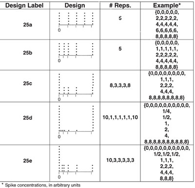
After steps 11–3 have been evaluated and the objectives for the calibration have been determined, the study can be designed. The critical decisions are the concentrations to include, and the number of replicates of each concentration. The first decision depends primarily on the range to be covered and the areas that need emphasis (e.g., low-DL and/or curvature regions). The second decision depends in large part on the precision needed in the various regions of the curve. It is not necessary that the same number of replicates be included for each concentration. However, replicates at multiple concentrations are needed in order to test a critical assumption of OLS; i.e., that the standard deviation is not increasing with concentration. A rule of thumb (but by no means a hard-and-fast recommendation) is to start with a 5-by-5 design (five levels, each with five replicates) and adapt as needed.
Some example designs are given in Table 1. As an exercise, the reader is invited to try evaluating each design in light of the above discussion and postulate why each example was structured as it is. The next article will discuss each layout and will present some actual calibration designs the authors have implemented. Happy trials!
References
- Coleman, D., Vanatta, L. Statistics in Analytical Chemistry: Part 4—Calibration: Uncertainty intervals. Am. Lab. 2003, 35(5): 60–2.
- Coleman, D., Vanatta, L. Statistics in analytical chemistry: A new American Laboratory column. Am. Lab.2002, 34(18): 44–5.
Mr. Coleman is an Applied Statistician, Alcoa Technical Center, MST-C, 100 Technical Dr., Alcoa Center, PA 15069, U.S.A.; e-mail: [email protected]. Ms. Vanatta is an Analytical Chemist, Air Liquide-Balazs™ Analytical Services, Box 650311, MS 301, Dallas, TX 75265, U.S.A.; tel: 972-995-7541; fax: 972-995-3204; e-mail: [email protected].