Statistics in Analytical Chemistry: Part 9—Calibration Diagnostics (continued)

The previous article (American Laboratory, Nov 2003) introduced the subject of calibration diagnostics. This protocol allows the analyst to decide if his or her proposed model is adequate for the calibration data. The seven basic steps are:

1. Plot response versus true concentration
2. Determine the behavior of the standard deviation of the response
3. Fit the proposed model and evaluate R²_adj
4. Examine the residuals for nonrandomness
5. Evaluate the p-value for the slope (and any higher-order terms)
6. Perform a lack-of-fit test
7. Plot and evaluate the prediction interval.

Steps 1 and 2 were discussed in part 8 of the series in the November issue. Steps 3 and 4 are explained this month.

Step 3: Fit the proposed model and evaluate R²_adj

Once the appropriate fitting technique has been determined, the proposed model can be fit to the data. Of interest is R², which is a measure of the proportion of total variation in the response (or any dependent variable) "explained" by the independent variable. (R² is calculated by taking the ratio of the model sum of squares to the total sum of squares. It should be noted that in the literature, R² is sometimes called the coefficient of determination.) If all of the response variation were explained by the model (a situation that never happens with real data), then R² = 1. If none of the variation were explained, then R² = 0 ( an equally rare occurrence); in this case, the proposed model would be no better than a zero-slope straight line through the mean of the response data.

Clearly, the closer R² is to 1, the better. However, for a given data set, the analyst must exert caution in comparing R² values for various models. It is not unusual for R² to rise just because another term is added to the model. Consequently, a more realistic statistic, R²_adj, is preferred. R²_adj penalizes R² for each explanatory (independent) variable used in the regression.

Even when using R²_adj, the analyst must exert caution in interpreting the value. Although the number is used extensively in deciding whether or not a calibration curve is adequate, it is perhaps the weakest of the seven diagnostic tools. In reality, R²_adj should be viewed as a number that gives the user a rough idea of the adequacy of the chosen model. (As will be illustrated in a future article, there are times when a calibration curve is quite adequate, even though it has an R²_adj value well below 0.99.)

Step 4: Examine the residuals for nonrandomness

When the proposed model is fit to the data, the accompanying residual plot should be generated as well. As was pointed out in installment 2 (American Laboratory, Nov 2002), the residual plot is one of the most useful tools in the calibration-diagnosis process. For each data point, the residual is the observed response minus the predicted response (i.e., the actual response obtained from the instrument minus the response that is calculated from the model at that particular true concentration).

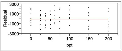
Figure 1 - Residual plot for an appropriate data model. The desired pattern is randomness (in the vertical direction) of the response about the zero line; at each concentration, this line (ideally) should pass through the mean of the responses. In reality, there probably will be some deviation from this goal and the user must decide how much nonideality is acceptable for the situation at hand.

The graph of these residuals should be a random scatter of points (in the vertical direction) about a horizontal line at zero. At each true concentration, the goal is to have the zero line intersect the mean of the responses. An example is given in Figure 1. If there is a definite nonrandom pattern (e.g., a parabola or sine wave) to the plot, then the proposed calibration model is not adequate. There is one exception to this statement. If the graph exhibits a trumpet shape, then the standard deviation of the responses is either increasing or decreasing with concentration. Assuming the pattern is otherwise random about zero, this situation is handled not by changing the model but by using weighted least squares (WLS) as the fitting technique. Even when the weights are applied, the residual pattern will remain trumpet-shaped; the response data will always have the same spread, no matter what the model or fitting technique (see Figure 2).

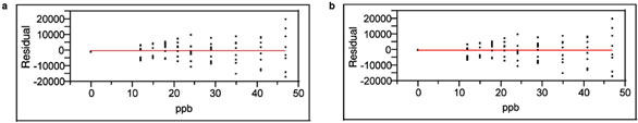
Figure 2 - a) Residual plot for an example data set, using ordinary least squares (OLS) to fit the chosen model. b) Residual plot using WLS for the same data set and same model as in (a). Note that there is virtually no difference between the two plots. At each concentration, the inherent response variation is not (and cannot be) changed when WLS is used.

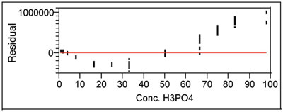
Figure 3 - Residual plot for a straight-line model applied to data that exhibit curvature.

A residual plot example for an obviously inadequate model (of response as a function of concentration) is shown in Figure 3. Instead of a straight line, a low-order polynomial may be needed; alternatively, perhaps the range of concentrations should be partitioned, and each interval fitted separately.

Mr. Coleman is an Applied Statistician, Alcoa Technical Center, MST-C, 100 Technical Dr., Alcoa Center, PA 15069, U.S.A.; e-mail: [email protected]. Ms. Vanatta is an Analytical Chemist, Air Liquide-Balazs™ Analytical Services, Box 650311, MS 301, Dallas, TX 75265, U.S.A.; tel: 972-995-7541; fax: 972-995-3204; e-mail: [email protected].