It’s important to realize that information gets filtered and distorted by the inherent behavior of a measurement process. In this column, we’ll ignore biases and look closely at the relationship between industrial process variation and measurement process variation.
Figure 1 shows an ideal process. At the far left we see starting materials entering the industrial process. A sample of the industrial process output becomes the input to the measurement process. The output of the measurement process becomes a description of how the industrial process appears to be behaving.
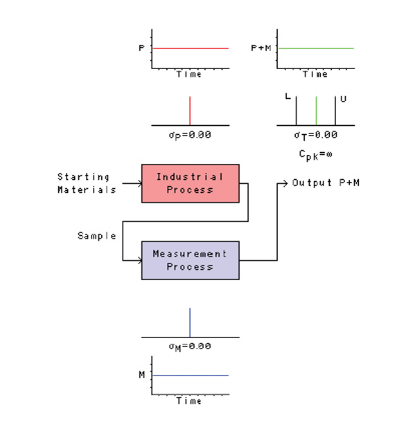 Figure 1 – The relationship between an industrial process and a measurement process.
Let’s assume that the industrial process is lined out, rock solid, no variation. This is depicted in the two small graphs above the industrial process. The upper graph shows the true values of the process output P plotted on the vertical axis as a function of time on the horizontal axis—the output P is absolutely constant. The lower graph shows the same thing in a different way: the true values of the process output P are now plotted on the horizontal axis with something related to their probability density on the vertical axis—again, there is no variation. Clearly, the inherent standard deviation of the industrial process σP is zero.
Now let’s look at the two graphs below the measurement process. The lower graph depicts the values obtained from repetitive measurements of a reference material M plotted on the vertical axis as a function of time on the horizontal axis. The upper graph shows the same thing in a different way—the measured values are now plotted on the horizontal axis. Clearly, the inherent standard deviation of the measurement process σM is zero.
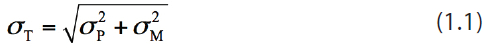
Here’s an equation that will be important to us. It illustrates how variations from more than one source combine to give the total variation. Note that the standard deviations aren’t additive—the variances (standard deviations squared) are additive:
If the industrial process has zero variation (σP = 0), and if the measurement process has zero variation (σM = 0), then the total variation of the measured industrial process will be zero (σT = 0). This is shown in the two graphs at the upper right of Figure 1, where the variation of the industrial process (P) and the variation of the measurement process (M) are combined (P+M). The upper graph shows the measured values as a function of time (rock solid), and the lower graph shows the same thing in a different way. Either way you look at it, there is no variation in the measured values.
But look closely at this lower graph. It also shows a lower specification L and an upper specification U separated by five units. In the last column in this series, L and U were specifications for the measurement process, but here they are specifications for the output of the industrial process. If the output is centered midway between the specifications, and if σT = 0, then Cpk is infinite! If this process behaves in the future as it has behaved in the past, then we will never encounter any measurements that indicate the industrial process is producing product that is out of specification. This is clearly what management wants to see.
But Figure 1 is unrealistic. Industrial processes don’t have zero variation. Measurement processes don’t have zero variation. So what does the real world look like? Let’s have some fun.
Figure 2 is the analytical chemist’s egotistical view of the world. In this universe, the measurement process has zero variation (we analytical chemists take great pride in our precision!), and all the observed variation is attributed to those darned engineers and their flaky industrial process.
 Figure 2 – An analytical chemist’s view of the world.
Although this view of the world is unrealistic (measurement processes don’t have zero variation), it actually represents what engineers would like us analytical chemists to provide—perfect measurements! If the measured values we gave them really did represent their industrial process exactly, then the engineers would have a good understanding of their process and its behavior, and they’d be able to see clearly the effects of any changes that they made. Hold that thought.
Figure 3 is the engineer’s egotistical view of the world. In this universe, the industrial process has zero variation (engineers know how to control things!), and all the observed variation is attributed to those untrained, inept, sloppy analytical chemists and their strange methods that they call measurement.
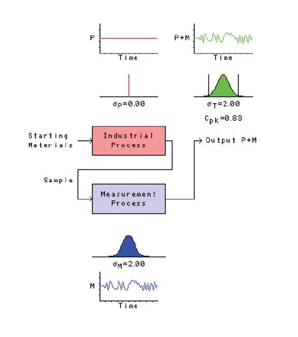 Figure 3 – An engineer’s view of the world.
This view of the world is also unrealistic (industrial processes don’t have zero variation), but it does illustrate a very important point for analytical chemists: excessive variation in the measurement process can prevent the engineers from understanding what their industrial process is actually doing. All they “see” are the graphs in the upper right. They don’t get to “see” the two graphs above the industrial process, the graphs that show what the industrial process is actually doing. As we discussed in a previous column, this can lead to “tampering” of the industrial process—observing changes that are actually a result of variation in the measurement process, thinking that these changes represent the behavior of the industrial process, and then taking inappropriate action on the industrial process. (We could devote a whole future column to a discussion of all the problems tampering causes.)
Figure 4 represents reality: industrial processes have variation, and measurement processes have variation. I’ve chosen this particular figure to illustrate two points.
 Figure 4 – The real world.
First, in my judgment, this is a picture of what a lot of biopharmaceutical companies are faced with. Biological measurements are often inherently highly variable—microorganisms (often the basis of many biological methods) exhibit exponential growth, and this makes the results fragile with respect to the timing of different steps in the analysis; very small volumes are used for analysis, and micro-pipettes don’t always perform as precisely or accurately as advertised; blunders are often made when samples are transferred to the top wells of 96-well plates, etc. I’m not saying bioassayists are untrained, inept, or sloppy—on the contrary! I have great admiration for their heroic efforts, given what they have to work with. It’s really tough to be a precise bioassayist!
But getting back to Figure 4, it’s my judgment that many biopharmaceutical manufacturing processes are probably inherently less variable than they appear. Biopharmaceutical engineers don’t get to see what good engineers they are, because the measurement variation masks the true tight behavior of their fine industrial processes.
My second point has to do with the apparent Cpk in this picture: σT = √(12 + 22) = √5 = 2.24, so Cpk = (L – U)/(3 × σT) = 5/(3 × √5) = 0.75 < 1, which suggests that the industrial process is not capable. In fact, the true Cpk of the industrial process is 5/(3 × σP) = 5/(3 × 1.00) = 1.67 > 1, which means the industrial process is inherently highly capable—it only appears to be incapable because of the obscuring measurement process variation.
I once read a talk from an awards ceremony for a statistician, during which he basically said to his colleagues, “Hey, guys. I just discovered that if you clean up your analytical methods, you can improve the Cpk of your industrial process without ever touching the process itself!” Well … yeah.
When I started graduate school at Purdue in 1966, we incoming analytical chemistry students were given a pep talk by Professor Herbert W. Laitinen,1 who was visiting from the University of Illinois. For some reason, I always remembered one of the things he said during that inspiring talk: “When you develop an analytical method, it should have only about one-tenth the variation you expect from the industrial process for which it will be used.” I never fully appreciated that statement until I started to look at process capability. If σP = 1 and σM = 0.1, then σT = √(12 + 0.12) = √1.01 = 1.005. The measurement process now has very little effect on the total variation!
This is illustrated in the simulation shown in Figure 5. The measurement process variation is one-tenth the industrial process variation, and the observed behavior of the industrial process (the green squiggly line at the very top right in the figure) matches almost exactly the true behavior of the industrial process (the red squiggly line in the top graph above the industrial process). Practically speaking, this is what the engineers need and want, the thought we’ve been holding from our discussion of Figure 2.
 Figure 5 – The world according to Laitinen.
Fifty years later, it’s good to appreciate that the pioneers in the field knew exactly what they were talking about. We should keep these concepts alive.2,3
References
- Laitinen, H.A. Chemical Analysis: An Advanced Text and Reference; McGraw-Hill: New York, N.Y., 1960.
- Hayes, J.D. Is it Process Variability or Measurement System Variability? http://virtual. auburnworks.org/profiles/blogs/is-it-process- variability-or-measurement-systemvariability
- Rodebaugh, B. Six Sigma in Measurement Systems: Evaluating the Hidden Factory,” slide 7; http://asq.org/cpi/2002/06/sixsigma- in-measurement-systems-evaluating- the-hidden-factory.ppt
Dr. Stanley N. Deming is an analytical chemist masquerading as a statistician at Statistical Designs, 8423 Garden Parks Drive, Houston, TX 77075, U.S.A.; e-mail: [email protected]; ; www. statisticaldesigns.com
UpdateCancel