The previous article (American Laboratory, Oct 2010) left off with two interesting questions: 1) How does an analyst decide whether a positive response for a blank is low enough to be ignored? and 2) Should an analyst ever consider constraining the y-intercept to zero (often called “forcing zero”)? This installment will address both of these queries, in order.
From the start, two points must be emphasized about blank responses. First, the concentration associated with a positive blank can never be estimated very reliably. By definition, there simply is no way to obtain response data at concentrations below the contamination level. Extrapolation (or its equivalent, the use of standard addition) is a very crude estimate at best.
Second, judgment calls about blank responses must be made within the context of the data set at hand. Any given calibration or recovery curve (or, for that matter, any regression line) has both bias and noise components. Recall the simple generic model from Part 2 of this series (American Laboratory, Nov 2002):
yi = f(xi) + εi + bias
where yi = measurement i (e.g., peak area); f(xi) = the function relating xi to yi; xi = true value (e.g., concentration); εi = “noise” or random error; and bias = systematic error (may not be constant with respect to xi).
Once an appropriate model and an adequate fitting technique have been found for a data set, the associated prediction interval reflects the precision (i.e., ε term) in those data. An indication of the bias is the y-intercept for the line. If this point is not “close” to zero, then there may be trouble (i.e., a blank response that is unacceptably high). How to make the call? Some sort of statistical interval is the needed measuring tool.
Since calibration and recovery curves are generated for the primary purpose of quantifying subsequent samples that are analyzed, a prediction interval is the correct choice. This pair of lines captures the noise and indicates the range within which the next prediction from the curve will lie (at the chosen confidence level). At x = 0, the blanks’ responses are statistically negligible (given the noise in the data) if the prediction interval contains zero. (When a true blank is analyzed and quantified via such a curve, the estimated concentration’s uncertainty width will almost always contain zero.)
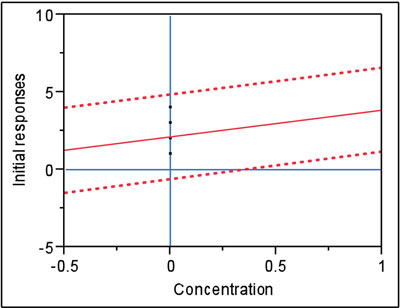
Figure 1 - In this example, the prediction interval (at 95% confidence) contains zero. Thus, there is no statistically significant difference between the blank’s positive response and zero.
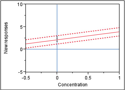
Figure 2 - In this example, the precision in Figure 1’s data has been tightened. Now the prediction interval (still at 95% confidence) does not contain zero. Therefore, there is a statistically significant difference between the blank’s response and zero.
Figure 1 is an example of the above situation. The data are the same as in Figure 1 (data set 1) in Part 40 (here, only the lower end of the curve is shown). As can be seen, the point (0,0) is included in the confidence interval (which is at 95% confidence). The position of the interval depends on the noise in the data and the values of the blank responses themselves. Thus, for these data and confidence level, the blank responses are not exerting a statistically significant bias.
What happens if the width of the interval shrinks (smaller is generally better)? One way to effect such a change is to decrease the confidence level, although that option may not be acceptable. Two other realistic (but probably more costly) possibilities exist: 1) improve the analytical method to make it more precise (e.g., develop a better sample-preparation protocol or obtain an improved instrument), or 2) analyze both calibration (or recovery) standards and samples in replicate, and work with averages. In either case, the noise in the data will shrink and the prediction interval will become narrower (given a fixed level of confidence). Such an example is shown in Figure 2. Since the original data were simulated, the responses for this second figure were obtained simply by shrinking the noise in the original data (the same regression line resulted). Note that with the decrease in noise, the prediction interval does not include the zero response at x = 0. Under these circumstances, the blank responses are significant from a statistical point of view and are cause for concern. Now the analyst should spend time trying to reduce the contamination, if at all possible.
What about the matter of “forcing zero”? In other words, if no analyte signal is obtained from a blank, or if no blank is available, should the regression process ever constrain the y-intercept to zero? In a word, no. Even if chemical or physical principles indicate y should be zero when x is zero, the data may not exactly follow the relationship because of problems such as bias or poor precision. (Keep in mind that something is going on at the zero-concentration level, even if instrument noise is the only source.)
Also, forcing zero involves extrapolation. As has been mentioned several times throughout this series of articles, extrapolating a curve beyond the study’s concentration range is not a sound practice. The user simply does not know how the responses will behave in these “black-hole” regions. Extrapolation is especially dangerous if the data exhibit curvature (i.e., if a quadratic or higher-order model is needed) or if weighted least squares is appropriate for the fitting technique (i.e., how does one handle the calculation of the weight in the “dataless” region?).
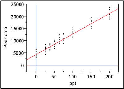
Figure 3 - Nitrite data fitted with a straight line, using ordinary-least-squares fitting. The y-intercept was not constrained to zero.
If a blank is not available, then forcing zero is a very risky undertaking. If the blank actually is contaminated with a measurable amount of analyte, then the constrained regression line’s slope will be altered, possibly to a significant degree. An illustration follows.
Recall the now familiar nitrite data, which have been investigated several times in this American Laboratory column. A straight line with ordinary-least-squares fitting is adequate for the regression line (see Figure 3). As can be seen, blanks were analyzed and positive responses were obtained. The y-intercept is well above zero (~4400). A full discussion of the diagnostics for this data set can be found in Part 12 (American Laboratory, Jul 2004).
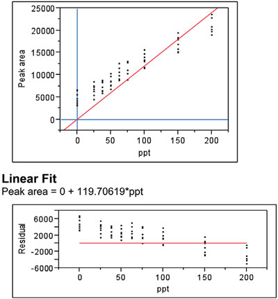
Figure 4 - Same as in Figure 3, except that the y-intercept has been constrained to zero.
Suppose blanks had not been available and it had been assumed that they were free of nitrite contamination, thereby leading the analyst to force zero. The result (along with the residual plot) is shown in Figure 4. Even a cursory look at the regression plot should alert the user to a problem, since the regression line fails even to intersect the vertical range of each group of points at six of the nine concentrations. The residual pattern makes the situation even clearer. There is definite bias in this model. This conclusion is supported by the p-value (<0.0001) for the lack-of-fit test.
In reality, there is nothing to gain by forcing zero. If the blank response is either very tiny or not measurable, then the y-intercept will be “near” zero when the nonconstrained regression curve is fitted. The confidence interval (at the user-chosen level of confidence) can be examined to determine if zero is included, thereby giving the analyst the information he or she needs to evaluate the blank’s influence on the regression line.
Lastly, a further comment is warranted on the matter of blanks that do not give a measurable signal. It is not wise to enter zeros as the response; the best protocol is to enter nothing. Zero does not have uncertainty, yet entering this digit for every blank will influence the position of the regression (although sometimes only slightly).
Mr. Coleman is an Applied Statistician, Alcoa Technical Center, MSTC, 100 Technical Dr., Alcoa Center, PA 15069, U.S.A.; e-mail: [email protected]. Ms. Vanatta is an Analytical Chemist, Air Liquide-Balazs™ Analytical Services, 13546 N. Central Expressway, Dallas, TX 75243-1108, U.S.A.; tel.: 972-995-7541; fax: 972-995-3204; e-mail: [email protected].