Measurement processes must be fit for use.1 In this column, we’ll develop some quantitative statistical descriptors of the capability of a measurement process to be valid for its intended purpose. To get started, we’ll need to review some fundamentals. You’ll need to master this material before we go on to the more interesting things, so don’t skip it. It’s generally agreed by theoreticians and experimentalists alike that replicate measurements follow a Gaussian distribution (see Figure 1). There are exceptions—low-mass spectral ion intensities follow a Poisson distribution, for example—but most measurements, or a transformation of these, exhibit approximately Gaussian behavior.
 Figure 1 – The standard normal (Gaussian) distribution showing that 99.73% of the measurements lie within ±3 standard deviations (
σ
) of the mean (μ
).The horizontal axis in Figure 1 is labeled in z units, which we’ll define in a minute. For the moment, consider this to be the measurement axis—the measurements are plotted from left to right, low to high. The unlabeled vertical axis in Figure 1 indicates the probability density. This is related to the probability of finding a given value along the horizontal axis. Clearly, values in the middle of the Gaussian distribution are more probable than values far to the left or far to the right.
Any segment of area under the curve is proportional to the fraction of measurements found within that area. For example, the fraction of measurements from the center of this symmetric curve out to positive infinity is 0.5; the fraction from negative infinity to z = –3 is very small, only 0.00135.
The center of the Gaussian curve, the most probable value, is the familiar mean. For an infinite number of measurements (something statisticians assume for this work), the mean is given the symbol μ. The distance from the mean to the inflection point on either side of the curve is the familiar standard deviation σ. This distance is shown by a short horizontal line in Figure 1.
So what’s a z value? If x represents a measurement, then:
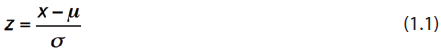
The units cancel out, so z values are unitless. The z value is a relative way of describing a measurement: it tells us how far the measurement x is from the mean in units of the standard deviation. Thus, a measurement that is one standard deviation above the mean has a z value of +1; a measurement with a z value of –2 is two standard deviations below the mean. Statisticians think in terms of z values, and we’ll have to, as well. Notice that 99.73% of the area under the Gaussian curve lies between z values of –3 and +3. This fact led Shewhart to choose so-called “three sigma limits” for the control charts we discussed in previous columns.
A capable process is usually defined as one for which at least 99.73% of the results lie between specifications.1 Look at Figure 1: if a lower specification L were at least three standard deviations below the mean, and if an upper specification U were at least three standard deviations above the mean, then at least 99.73% of the measurements would lie between these specifications. We’ll define the distances of the specifications from the mean as zL and zU:
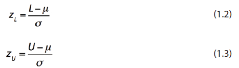
Clearly, if zL is at least as negative as –3 and, at the same time, zU is at least as positive as +3, then the process will be capable.
But what are these specifications, L and U? Are they product specifications? No, absolutely not. They are specifications for the measurement process.
 Figure 2 – Results for a measurement process that is not capable:
 μ
= population mean = 0.98; σ
= population standard deviation = 0.03; L
= lower measurement specification limit = 0.95; U
= upper measurement specification limit = 1.05; z
L = –1.00; z
U = +2.33; ST
= 3.333; Cp
= 0.56; C
pk = 0.33.Let’s go to the pharmaceutical industry for an example. Suppose a regulatory agency requires the amount of active ingredient in a pharmaceutical product to lie between 0.90 and 1.10 of the label claim. You’re thinking, “Aha! If 99.73% of the measurements lie between 0.90 and 1.10 of the label claim, then the measurement process is capable.” That would be true if there weren’t variation in the production process itself, but we have to allow the engineers some leeway. Suppose we agree to split the variation equally between the engineers and the analysts. That means the engineers can produce material between 0.95 and 1.05 of the label claim, and when we measure one of these extreme batches our measurements must lie between 0.90 and 1.10 of the label claim. For these extreme batches, our measurements can be wrong by at most 0.05 on the low side and at most 0.05 on the high side, that is, the specifications for our measurement process are ±0.05 on the measurement axis. Thus, repetitive measurements of a reference standard (for which the amount is taken to be 1.00) must lie between 0.95 and 1.05 at least 99.73% of the time for our measurement process to be capable.
For the biased measurement process shown in Figure 2, μ = 0.98, σ = 0.03, zL = (0.95 – 0.98)/0.03 = –1.00 and zU = (1.05 – 0.98)/0.03 = +2.33. It’s clear from these numbers that the process isn’t capable: zL is not as negative as –3 and 15.87% of the measurements are below L; zU is not as positive as +3 and 0.99% are above U. Thus, only 83.14% of the measurements lie within specifications … and the process is not capable.
The specified tolerance (ST) is a useful process capability index2-4:
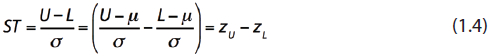
The specified tolerance must be 6 or greater for the process to have the possibility of being capable. This is an “elbow room” concept: if zL has to be at least as negative as –3, and if zU has to be at least as positive as +3, then there must be at least six standard deviations between L and U. In our example, zU – zL = 2.33 – (–1.00) = 3.33, which is less than 6, so the process isn’t capable.
In fact, this measurement process, as it exists, can never be capable. There isn’t enough room between L and U. Figure 3 shows a best-case situation where the mean is centered between the two specifications. Now zL = –1.67 and zU = +1.67 (ST is still equal to 3.33), and 90.50% of the measurements will lie between the specifications. This is better than 83.14%, but the fraction of measurements between specifications can never be greater than 90.50%.
 Figure 3 – Results for a measurement process that is not capable:
 μ
= population mean = 1.00; σ
= population standard deviation = 0.03; L
= lower measurement specification limit = 0.95; U
= upper measurement specification limit = 1.05; z
L = –1.67; z
U = +1.67; ST
= 3.33; C
p = 0.56; C
pk = 0.56.Curiously, statisticians have created a process capability index, Cp, which expresses the same information contained in ST: Cp = (U – L)/(6σ) = ST/6 = (zU – zL)/6. Thus, if Cp is greater than or equal to 1, the process can be capable. I’m amused by this unnecessary capability index: stating that Cp ≥ 1 is the same as stating that ST ≥ 6. In my opinion, ST expresses a concept that is easily interpreted (“elbow room”); Cp is a step removed from that concept.
If there isn’t enough elbow room between specifications, what has to be done? The standard deviation must be reduced. And, as we discussed in the last column, this is tough. It isn’t easy to reduce the variation of a measurement process, but you’ll have to find some way to do it (or get the engineers to tighten up their process to give you more room, though this is unlikely).
 Figure 4 – Results for a measurement process (green) that is capable:
 μ
= population mean = 0.98; σ
= population standard deviation = 0.01; L
= lower measurement specification limit = 0.95; U
= upper measurement specification limit = 1.05; z
L = –3.00; z
U = +7.00; ST
= 10.00; C
p = 1.67; C
pk = 1.00. See text for a discussion of the other (mostly red) Gaussian distribution for which C
p is also equal to 1.6.Figure 4 shows an improved, yet still biased, measurement process with a mean μ = 0.98 and a reduced standard deviation σ = 0.01 (the green Gaussian in the figure). Now the Cp = 1.67, so there is enough room for this measurement process to be capable … and it is capable: zL = –3 and zU = +7, ST = 10.
Look at the measurement process represented by the mostly red Gaussian curve in Figure 4. It, too, has a standard deviation of 0.01, so the Cp for it is also 1.67. But this process certainly isn’t capable. The process could be capable if it had less bias. It is for this reason that Cp has been called the “process potential index.” We need still another process capability index to take into account the “centering” of the distribution with respect to the specifications.
This is the Cpk, the centered process capability index. It is a measure of the distance from the mean to the nearest specification and should be a positive number:
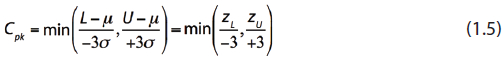
 Figure 5 – Results for a measurement process that is highly capable:
 μ
= population mean = 1.00; σ
= population standard deviation = 0.0083; L
= lower measurement specification limit = 0.95; U
= upper measurement specification limit = 1.05; z
L = –6.00; z
U = +6.00; ST
= 12.00; C
p = 2.00; C
pk = 2.00. This is “six-sigma” quality.If Cpk ≥ 1.00, the process is capable. For the green Gaussian curve in Figure 4, Cpk = 1.00 because zL = –3.00 and zU = +7.00. The process is close to L because of the bias, but it is far enough away from L that it is still capable. For the mostly red Gaussian curve in Figure 4, zL = –12.00 and zU = –2.00, and Cpk = –0.67, clearly not greater than 1.00, so this process isn’t capable. But we knew this already, because, although zL is at least as negative as –3, zU is not at least as positive as +3.
Figure 5 illustrates the original concept of “six-sigma” quality—the mean is at least six standard deviations from the nearest specification (ST ≥ 12.00, Cpk ≥ 2.00). The probability of getting a measurement beyond the specifications is vanishingly small. Manufacturers like this concept; perhaps analytical chemists should, too.
One last point. In the real world, we don’t have an infinite number of measurements, so our estimates of μ and σ are a bit fuzzy. As a result, estimated values of zL, zU and the calculated capability indexes are also a bit fuzzy. The more replicate measurements the better, but if you’re concerned about this, see a real statistician.
I thank Tim Schofield for his many helpful comments.
References
- Scherkenbach, W.W. The [William Edwards] Deming Route to Quality and Productivity: Road Maps and Roadblocks, 1st ed.; ASQC Quality Press: Milwaukee, Wis., 1986 [ISBN 0-941893-00-6].
- Kotz, S. and Johnson, N.L. Process Capability Indices; Chapman and Hall/CRC: London, 1993 [ISBN 0-412-54380-X].
- NIST/Sematech. What is Process Capability?; http://www.itl.nist.gov/div898/handbook/pmc/section1/pmc16.htm
- Steiner, S.; Abraham, B. et al. Understanding Process Capability Indices; http://www.stats.uwaterloo.ca/~shsteine/papers/cap.pdf
Dr. Stanley N. Deming is an analytical chemist masquerading as a statistician at Statistical Designs, 8423 Garden Parks Dr., Houston, Texas 77075, U.S.A.; e- mail: [email protected]; www.statisticaldesigns.com