Use of Weighted Least Squares and Confidence Band Calibration Statistics to Find Reliable Instrument Detection Limits for Trace Organic Chemical Analysis

The Appendix below provides theoretical background to a shorter version of the article that appears in the September issue. Following the Appendix is the full version of the article.

Appendix

Introduction

Instrument detection limits (IDLs or x_D) obtained from applying either ordinary least squares/confidence band calibration statistics (OLS/CBCS) or weighted least squares/confidence band calibration statistics (WLS/CBCS) are based on first establishing confidence or prediction intervals that surround the OLS or WLS regressed calibration curve. Second, the y-intercept y₀ is identified as the apex of a normal (Gaussian) distribution at x = 0 (amount or concentration of the chemical analyte of interest expressed as pg or pg/μL and assumed free of error). Third, the critical instrument response y_C as determined with a t distribution with α = 0.05 is established. Fourth, a horizontal line (refer to Figure 1) is drawn from y_C to the calibration line to establish the analyte’s critical decision level x_C. Fifth, continuing along the horizontal line to the lower confidence limit y_L, where β can be set to 0.05, serves to establish the chemical analyte’s x_D or IDL. Figure 1 depicts the important parameters.¹

Figure 1 ‒ Finding the critical instrument response y_C and critical amount or concentration x_C while minimizing Type 1 errors for OLS/CBCS and for WLS/CBCS.

The intersection of the upper confidence limit with the y axis at y_C, where x = 0, corresponds to the highest signal that could be attributed to a blank 100 (1-α)% of the time. In other words, the critical instrument response y_C is set at α = 0.05 such that 95% of all measurements are to be found below this critical value. This is represented by a one-sided t distribution of instrument responses. It is evident that the critical instrument response y_C is established such that the probability of making a Type 1 (false positive) error is minimized at α = 0.05.²

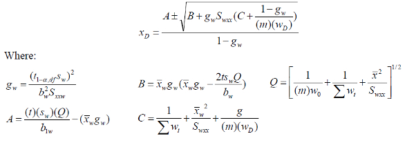
Equations for the critical instrument response for only WLS/CBCS are given below:

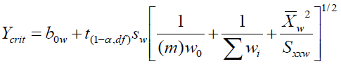
Where:
y_crit is the critical instrument response
b_0w is the y-intercept from the WLS regression
t_(1‒α,df) is the student’s t for a one-sided hypothesis test for a specific number of degrees of freedom, df, where df = N-2 with N = the number of x,y data points used in the calibration
s_w is the standard deviation in the weighted y residuals for a WLS regression and is found as follows:

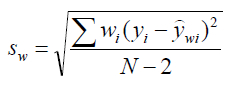
Where:
w_i is the weight factor for the ith data point in the calibration
y_i is the instrument response for the ith data point
N is the number of x,y data points in the calibration
ŷ_wi is the calculated weighted instrument response that corresponds to the ith data point obtained from application of the weighted least squares equation:

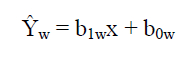
Where:
ŷ_w is the instrument response for the WLS regression
b_1w is the WLS/CBCS regression slope
x is the known amount (pg) or concentration (pg/μL) for a given analyte (assumed free of error)

The corresponding critical decision level x_C is calculated according to:

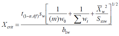
Where:
x_crit is the critical amount (pg) or concentration (pg/μL), also noted as x_C
b_1w is the WLS/CBCS regression slope
m is the number of post-calibration sample replicates
w₀ is the weight at x = 0
Σw_i is the sum of the weights over i x,y data points used to construct the WLS regression
x̄ is the mean of N x values used to construct the WLS regression
S_xxw is the weighted sum of x squared mean deviations

The coefficient of determination r² is an important measure of how well the WLS regressed line fits to the experimental calibration points. Values >0.9900 have become an important criterion in trace quantitative analysis. r² is calculated in the spreadsheet by squaring the correlation coefficient r. r is calculated in the spreadsheet for the WLS/CBCS regression according to:

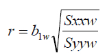
Where S_yyw is the weighted sum of y squared mean deviations

Calculation of x_C establishes a critical amount (pg) or concentration (pg/μL) level. This critical level x_C, defined over 40 years ago, is a decision limit at which one may decide whether the result of an analysis indicates detection.^3,4 x_C accounts only for Type 1 (false positive) error and infers that the analyte of interest can be detected but not reliably quantitated. Type 2 error (false negative) has not been minimized at this point.

Estimating the instrument response limit y_D and instrument detection limit x_D and calculating the instrument detection limit x_D while minimizing Type 2 (false negative) errors
Refer to Figure 1. The intersection of y_C with the lower confidence limit at y_L corresponds to the lowest signal that could be attributed to an analyte amount or concentration x_D 100(1-β)% of the time. This is represented by a t distribution of instrument responses with a one-tailed β for y at x = x_D.

Equations for the instrument detection limit (IDL) denoted as x_D and obtained from the literature for WLS/CBCS are shown below^1,5:

Conclusion

This Appendix provides the mathematics that underlie application of a spreadsheet to quickly and conveniently calculate critical decision levels, x_C and reliable IDLs, x_D, based on application of WLS/CBCS. The literature references suggest that these ideas have more than a 40-year lifespan.

The spreadsheet introduced in the print version incorporates all of the above mathematical equations to calculate the important parameters from application of WLS/CBCS. In addition, discrimination intervals that surround an interpolated value for the amount or concentration x for a given instrument response y can be calculated.⁵ Discrimination intervals provide important statistical information by stating the degree of uncertainty obtained for an interpolated value, x, for a chemical analyte in an environmental or clinical sample.

References

1. Budge, J.; MacTaggart, D. et al. Realistic detection limits from confidence bands. J. Chem. Educ. 1999, 76, 434.
2. Loconto, P.R. Trace Environmental Quantitative Analysis, 2nd ed.; CRC Press, Taylor and Francis: Boca Raton, London, New York, 2006, Chapter 2. A comparison of blank statistics vs confidence band calibration statistics to find detection limits is presented. In addition, many other aspects of calibration, verification and the statistical treatment of analytical data are introduced.
3. Currie, L. Limits for qualitative detection and quantitative determination. Anal. Chem. 1968, 40, 586.
4. Hubaux, A. and Vos, G. Decision and detection limits for linear calibrations curves. Anal. Chem. 1970, 42, 849.
5. MacTaggart, D. and Farwell, S. Analytical use of linear regression. Part I: regression procedures for calibration and quantitation. J.AOAC Int. 1992, 75, 594.

Complete version of article:

Use of Weighted Least Squares and Confidence Band Calibration Statistics to Find Reliable Instrument Detection Limits for Trace Organic Chemical Analysis

Most analog signals derived from element-specific and mass spectrometric detectors interfaced to gas and liquid chromatographs are electronically digitized. Today, chemists who use analytical instruments must contend less with analog signal noise and more with data acquisition rate and bunching factors. Using a value with 3× the standard deviation in the signal noise to calculate a chemical analyte’s limit of detection (LOD) is not adequate in the digital age.

Zorn et al. showed that polychlorinated biphenyls (PCBs) exhibit a non-constant variance (heteroscedasticity).¹ They compared unweighted or ordinary least squares (OLS) with weighted least squares (WLS) regression parameters. They found that the y-intercept of the regressed calibration curve was moderately affected, the slope of the regressed calibration curve was unaffected, and that residual standard deviation decreased significantly.

Plots of instrument response versus analyte concentration (pg/μL or ppb) using WLS/CBCS (in general) show that the width of prediction intervals are much smaller at or near the low end of the calibration and much larger near the high end of the calibration. Lower and more accurate x_C (critical concentration) and x_D (concentration at the lowest level of detection or IDL) result.

Heretofore, most derivations of x_D yielded an equation whereby x_D is set equal to an equation that includes x_D.² A breakthrough occurred when MacTaggert and Farwell derived an equation for x_D without x_D appearing on the right side of the equation.³ Subsequently, similar algebraic manipulations to calculate x_D for OLS and WLS regressions based on confidence band calibration statistics (CBCS) were achieved.⁴

This paper demonstrates how the equations for both OLS/CBCS and WLS/CBCS, drawn from the literature and incorporated into a spreadsheet, are used to calculate x_C and x_D. The same calibration data were used to compare results from applying the mathematics for OLS/CBCS to those obtained from applying the mathematics for WLS/CBCS for several organic chemical analytes of interest to public health. These included upper and lower prediction limit plots developed for the following organic compounds: ricinine and abrine quantitated using LC/MS/MS (4-hydroxy-3-nitro); phenyl acetic acid (HNPAA) quantitated using LC/MS/MS; and selected toxaphene congeners of environmental interest quantitated using gas chromatography and electron capture negative ion mass spectrometry (GC/ECNI/MS).

Experimental

Ricinine/abrine analysis

A Prominence Series HPLC system (Shimadzu Scientific Instruments, Columbia, Md.) was interfaced to an API 4000 triple quadrupole mass spectrometer with a Turbo V IonSpray (electrospray) source (Applied Biosystems/Sciex, Framingham, Mass.). Data was collected and analyzed using Sciex Analyst (version 1.5.1) software. A 10-μL sample was injected onto a Synergi Polar RP 2.1 mm × 100 mm, 2.5-μm particle-size column (Phenomenex, Torrance, Calif.) with an oven temperature of 40 ºC and flow rate of 0.3 mL/min; run time was 8 minutes. Mobile phase under gradient elution was as follows: solvent A—5% methanol in water + 5 mM formic acid; solvent B—acetronitrile + 5 mM formic acid, 0% B for 0.5 minutes after injection, then 0%B to 40%B from 0.5 minutes to 4.0 minutes; 40%B to 0%B from 4.0 minutes to 8.0 minutes.

HNPAA analysis

The same instrument and data system were used as above. A 10-μL sample was injected onto an Ascentis C8 2.1 mm × 50 mm, 3-μm particle size column (Supelco, Bellafonte, Penn.); oven temperature was 35 ºC, flow rate was 0.2 mL/min (flow increased to 0.6 mL/min from 3 to 5.5 minutes) and run time was 6 minutes. The mobile phase was 65:35 acetonitrile/water + 0.1% acetic acid.

Toxaphene congeners analysis

The GC/MSD (mass selective detector) operating in selective ion monitoring (SIM) mode and incorporating a CIS 4 programmed temperature vaporizer inlet (Gerstel, Linthicum, Md.) was interfaced with ChemStation software (Agilent Technologies, Wilmington, Del.) for chromatographic control, data acquisition and storage. Methane gas was introduced directly into the ion source to achieve dissociative electron-capture negative ions. Separation of toxaphene congeners was done using a DB-XLB (30 m × 0.25 mm × 0.25 μm film thickness) capillary column (Agilent) with a multistep oven temperature ramp. An MPS 2 dual-rail robotic autosampler system (Gerstel) was mounted on top of an Agilent 6890/5973N inert GC/MSD. The MPS 2, integrated with ChemStation software, is capable of liquid delivery. Using the CIS 4 inlet with cryo-trapping capability, a large-volume injection (LVI) of 10 μL was made without appreciable chromatographic band broadening.

Brief descriptions of sample preparation for ricinine/abrine, HNPAA and toxaphene congeners are given below.

Results and discussion

The paradigm shift introduced above is best realized graphically. Figure 1 depicts the blank statistics model. Normal (Gaussian) distributions for instrument responses are shown for the blank, LOD and LOQ (limit of quantification), where S is the standard deviation in baseline noise. It is evident that the risk of making a Type I error (shown as α) is minimized, while the risk of making a Type II error (β) is not minimized. Figure 1 illustrates the intrinsic limitation of calculating IDLs based on blank statistics.

Figure 1 ‒ Plot of the frequency distribution of instrument responses (y-axis) vs amount or concentration (x-axis) for a specific analyte (blanks statistics model). This model defines the LOD as 3× standard deviation in the mean blank signal. A limit of quantitation is defined as 10× standard deviation in the mean blank signal.

In contrast to Figure 1, Figure 2 displays the confidence band calibration statistical model for calculating a decision limit x_C, whereas α is minimized and β is not, and a detection limit x_D with both α and β minimized.⁵ As shown in Figure 2, the critical instrument response y_C is a statistical measure drawn from the intersection of the upper prediction limit with the y-axis in such a way that a Type I risk is minimized with α = 0.05 graphically. Figure 2 depicts the importance of the critical instrument response y_C in establishing x_C and x_D.

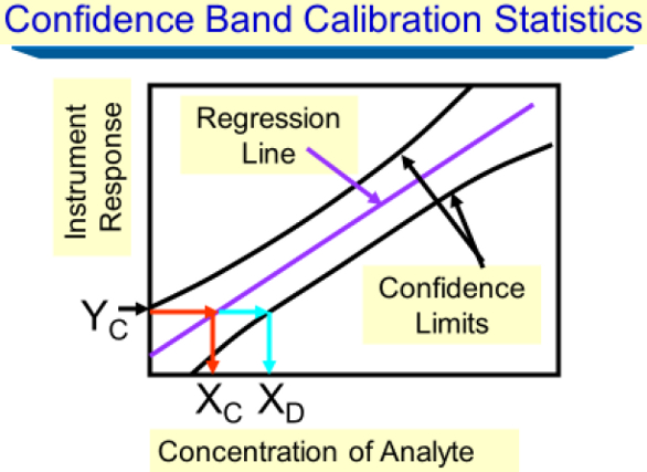Figure 2 ‒ Plot of instrument response vs analyte amount or concentration for the OLS approach to calculating x_C and x_D (confidence band calibration statistics model). A critical response y_C is defined as the position on the y-axis where the upper confidence (prediction) limit meets the ordinate when x = 0. Graphically, moving horizontally from y_C to the position on the calibration plot, then vertically down to the abscissa, yields the critical concentration, x_C. Continuing to move horizontally to the lower confidence (prediction) limit, and then moving vertically down to the abscissa, yields the instrument detection limit, x_D.

The prediction limits that shroud the calibration curve shown in Figure 2 were drawn based on OLS, while a similar WLS regression plot would show a significant narrowing of the prediction interval near x = 0 and a significant widening of the prediction interval near the high end of the calibration.

Comparing Figures 1 and 2, it is evident that the LOD (blank statistical model) is only near the decision limit x_C (CBCS model). The LOD will always be lower than the x_D (CBCS model) and this may be the reason analysts favor the former when reporting detection limits.

A spreadsheet using previously published mathematical equations allows users to quickly implement WLS/CBCS to calculate IDLs for trace organics.⁴  Table 1 shows the upper left portion of the spreadsheet used to calculate the critical or decision limit x_C and the IDL x_D for HNPAA based on WLS/CBCS. Note that x_i = ppb HNPAA (x_i values are assumed to be free of error) and y_i = ratio of abundance at m/z HNPAA to the abundance m/z for the internal standard (ISTD), a ¹³C-labeled HNPAA. The user inputs only x,y calibration data for each of N calibration levels.

Table 1 ‒ Upper left portion of the spreadsheet used to calculate IDLs based on WLS/CBCS for the calibration of HNPAA by LC-MS-MS

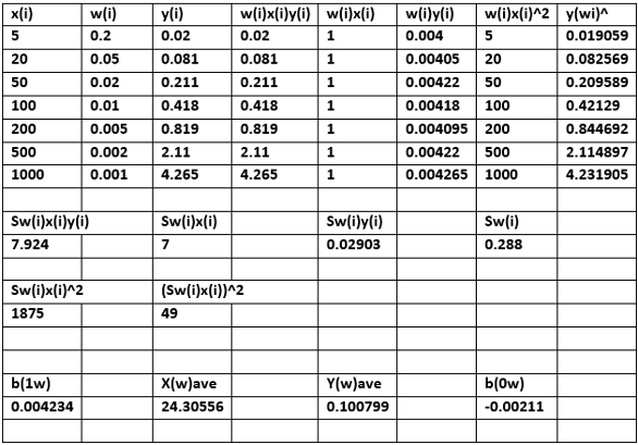
Incorporation of ISTDs is essential when using mass spectrometers to eliminate systematic errors when conducting trace organics quantitative analysis. The user must also input student’s t for one-tailed hypothesis testing, α = 0.05 (95% confidence level) or α= 0.01 (99% confidence level); the number of degrees of freedom less two or df = N-2; and student’s t for two-tailed hypothesis testing, α = 0.05 or 0.01, df = N-2.

A weight model using inverse concentration, which is widely used in commercial chromatographic software, was utilized for all chemical analytes for the WLS/CBCS applications reported here. The mathematical equations used for WLS/CBCS require a weight factor (w₀) of x = 0. A weight factor at the detection limit w_D was also required from the mathematical equations.⁴ A plot of w_i =1/x_i was needed to more accurately estimate w₀, while w_D was estimated at or near the numerical value for the lowest calibration standard. The user can choose a weight model other than inverse concentration in the spreadsheet.

The generated output, e.g., y_C, x_C and x_D, is based on application of WLS/CBCS. Additional outputs include the weighted slope b_1w; the weighted y-intercept b_0w and the important standard deviation in the weighted y residuals, s_r^w.

Table 2 shows one set of x,y calibration data for ricinine quantitated using LC/MS/MS. Six calibration standards from 0.3 ppb to 300 ppb were spiked into equal volumes of urine. The ISTD (¹³C-labeled ricinine) was spiked into each of the six calibration standards. The x,y data was entered into the OLS/CBCS spreadsheet and the parameters (defined in column 3 of Table 2) were generated, as shown in column 4. The same x,y calibration data was also entered into the WLS/CBCS spreadsheet and the important parameters were generated (see column 5). Ricinine and abrine were baseline separated.

Table 2 ‒ Calibration data and comparison of OLS/CBCS vs WLS/CBCS for ricinine in urine using LC/MS/MS

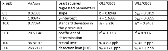
Molecular structures for ricinine and abrine are shown in Figure 3. These highly toxic organic compounds were isolated from human urine using a 96-well plate incorporating a conditioned polymeric reversed-phase solid-phase extraction (RP-SPE) sorbent. After passing the sample through the RP-SPE sorbent, the sorbent was washed and eluted with acetonitrile. The eluent was evaporated to dryness and reconstituted to a precise final volume with water. The analytes were quantitated using LC/MS/MS. As can be seen, the OLS slope b and WLS slope b_1w are comparable. The WLS y-intercept b_0w is an order of magnitude or more lower than the OLS y- intercept b₀. The WLS standard deviation in the y-residuals s_r^w is an order of magnitude lower that the OLS standard deviation in the y-residuals s_r. Correlation coefficients (r²) are comparable. The WLS critical limit x_C is an order of magnitude lower than the OLS critical limit x_C. The WLS/CBCS x_D is an order of magnitude lower than the OLS/CBCS x_D. The lowered y-intercept and standard deviation in the y-residuals are the principal factors that lead to a lowered IDL using the same calibration data.

Figure 3 ‒ IDLs were calculated for the molecular structures of these organic compounds. a) Ricinine, b) abrine, c) a hepta and an octa-chlorobornane, d) (4-Hydroxy-3-nitro) phenylacetic acid.

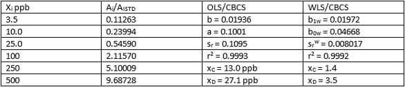
Table 3 compares OLS/CBCS and WLS/CBCS for one set of calibration data for abrine. Again, the slopes and r² values are comparable. The y-intercepts and standard deviations in the y-residuals (s_r vs s_r^w) are significantly lower. These differences lead to much lower x_C and x_D when applying WLS/CBCS to the same calibration data set.

Table 3 ‒ Calibration data and comparison of OLS/CBCS vs WLS/CBCS for abrine in urine using LC/MS/MS

OLS/CBCS and WLS/CBCS for two different calibration sets of data for HNPAA are compared in Tables 4 and 5. Again, comparable least-squares slopes and r² values are evident, while y-intercepts and s_r^w values using WLS/CBCS are much lower than equivalents using OLS/CBCS. This difference translates into significantly lower x_C and x_D values. Results for Tables 4 and 5 reveal nearly identical values for x_C and x_D.

Table 4 ‒ Calibration data and comparison of OLS/CBCS vs WLS/CBCS for HNPAA in urine using LC/MS/MS

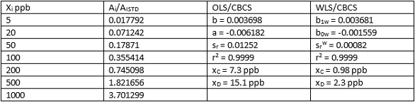
Table 5 ‒ Calibration data and comparison of OLS/CBCS vs WLS/CBCS for HNPAA in urine using LC/MS/MS

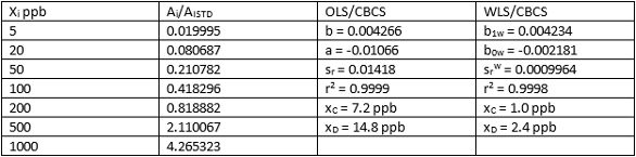
Figure 4 shows a WLS regression calibration plot shrouded within prediction limits for one calibration for the analyte HNPAA, the molecular structure of which is also shown in Figure 3. HNPAA, a metabolite found in human urine due to exposure to explosives such as TNT, was diluted with water and filtered using a 96-well plate RP-SPE disk to remove interferences. The analyte now in the filtrate was adjusted to a precise final volume and quantitated using LC/MS/MS. Calibration standards, including internal standards for HNPAA, were prepared in the blank sample matrix and underwent sample preparation.

Figure 4 ‒ Plot of WLS calibration and prediction limits for HNPAA. Note the gradual increase in the confidence (prediction) interval across the calibration, i.e., from low to high concentration.

The standard deviation in the weighted y residuals s_w for HNPAA was found to be much lower when compared to ricinine and abrine. This low value contributes significantly to lower IDLs when using WLS. Note the relative “tightness” of the prediction intervals (gray and red lines) that shroud the low end of the WLS calibration (blue line). Also note the gradual widening of the prediction interval at the high end of the calibration. This is consistent with the heteroscedastic behavior exhibited by many organic compounds.

Table 6 lists the nomenclature for the eight toxaphene congeners and one surrogate. A representative molecular structure for two toxaphene congeners is shown in Figure 3. IDLs using WLS/CBCS were applied to the eight toxaphene congeners and one surrogate. The goal was to calculate IDLs at ultratrace levels, and to establish lower IDLs using the LVI technique.

Table 6 ‒ Eight toxaphene congeners and one isotopically labeled toxaphene congener

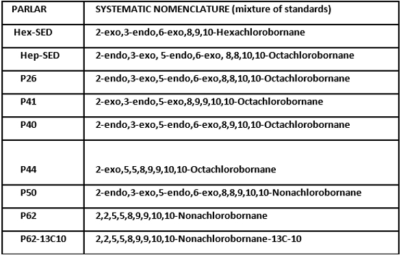
The eight congeners and surrogate listed in Table 6 were isolated and recovered from human serum and from Great Lakes fish tissue using conventional liquid‒liquid extraction (LLE) followed by silica gel cleanup, fractionation and subsequent extract concentration. Fish tissue was analyzed with and without the outer skin. The tissue was homogenized before the initial LLE. Calibration standards incorporating internal standards were prepared independent of the sample matrix and were not taken through sample preparation. Following each calibration, an IDL was found for each toxaphene congener and for the ¹³C-P62 surrogate.

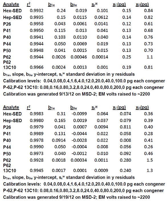
Table 7 summarizes results from two calibration sets for the eight toxaphene congeners and one ¹³C-P62 surrogate listed in Table 6. Calibration data was subjected to WLS/CBCS using the spreadsheet. A GC/ECNI/MS incorporating automated sample handling using cryo-trapping and LVI (10 μL) was used to generate the data. All nine analytes were baseline separated on a 30 m × 0.25 mm × 0.25 μm DB-XLB capillary column (Agilent Technologies) and exhibited excellent peak shape and narrow peak width. The instrument was calibrated in terms of pg injected each analyte. Dividing pg by 10 μL yields pg/μL or ppb each analyte. Isotopically labeled ¹³C-P-62 was added to every standard and sample as a surrogate. IDLs were very low, e.g., for Hex-SED, the calibration on 9/13/12 was 84 ppt (0.084 ppb); on 9/19/12 it was even lower—36 ppt (0.036 ppb). The results shown in Table 7 suggest that the magnitude of the weighted y-residuals srw (assuming all other WLS parameters were equal) contributed most to achieving very low IDLs. The mathematics are such that x_C is independent of x_D.

Table 7 ‒ Results from applying WLS/CBCS to two different calibration sets for toxaphene congeners and for one surrogate using GC/ECNI/MS

Conclusion

IDLs obtained using WLS/CBCS were significantly lower than those obtained using OLS/CBCS for a selected number of organic chemical analytes of importance to public health and the environment. The key parameters responsible for the differences from the mathematics were identified and discussed.

References

1. Zorn, M.; Gibbons, R, Sonzogni, W. Weighted least squares approach to calculating limits of detection and quantification by modeling variability as a function of concentration. Anal. Chem. 1997, 69, 3069.
2. Oppenheimer, L.; Capizzi, T.,Weppleman, R., Mehta, H. Determining the lowest limit of reliable assay measurement. Anal. Chem. 1983, 55, 638.
3. MacTaggart, D. and Farwell, S. Analytical use of linear regression. Part I: regression procedures for calibration and quantitation. JAOAC Int. 1992, 75, 594.
4. Budge, J.; MacTaggart, D. et al. Realistic detection limits from confidence bands. J. Chem. Educ. 1999, 76, 434.
5. Einax, J.; Zwanziger, H., Geiss, S. Chemometrics in Environmental Analysis, Chapter 2. http://onlinelibrary.wiley.com/book/10.1002/352760216X

Dr. Paul R. Loconto recently retired from the Michigan Department of Community Health, Bureau of Laboratories, where he focused on implementing existing methods and developing new analytical methods to isolate and recover trace organic analytes from water, serum, blood, urine, and fish tissue. He can be reached at 517-347-4195; e-mail: [email protected]. The author thanks Paul Gulyas for the LC/MS/MS data, Michael Stagliano for information on experimental LC/MS/MS and Robert L. Stevenson for his thoughtful and constructive critique. Support was provided by the Michigan Public Health Institute, Okemos; the Michigan Department of Community Health, Bureau of Laboratories, Lansing; the Department of Health and Human Services; and Emergency Preparedness and Response, the Centers for Disease Control and Prevention.