Spectrometer calibration accuracy is of critical importance for many optical characterization techniques such as Raman spectroscopy and interferometry.1–3 Typically, a calibration lamp is used for spectrometer calibration. Calibration lamps provide distinct, well-defined lines at a known wavelength, and these are assigned to the pixel indices of the detector. However, for small spectral ranges, where only a small number of calibration lines are available, the calibration becomes inaccurate. This article describes the principles of a high-precision calibration method that utilizes a Fabry-Perot multilayer structure, providing multiple sharp calibration peaks over the full spectrometer range.
Calibration methods
In most cases, spectrometers are calibrated using conventional calibration lamps. Although this method is simple to use, it has some restrictions; these are described below.
Conventional calibration lamps
A calibration lamp illuminates the spectrometer, and the positions—i.e., pixel indices (p) of the calibration lines of known wavelengths (λ)—are measured. A quadratic or higher-order-polynomial fit to the data (wavelengths [λ] at positions [p]) yields the calibration function sought—λ(p). Calibration lamps (e.g., Hg/Ar lamps) provide emission lines at a given wavelength. As a rule, there are broad wavelength regions with no peaks, which lead to limited calibration accuracy. Furthermore, a fit of higher-polynomial degree (N>3) requires a certain number of calibration lines, which might be limited in, e.g., spectrometers with small spectral ranges. The conventional method is less reliable, particularly for miniature spectrometers, which exhibit strongly nonlinear light dispersions. The calibration method described here solves this problem by using an additional optical element that generates a set of evenly distributed reference lines for any given range.
Fabry-Perot reference filter
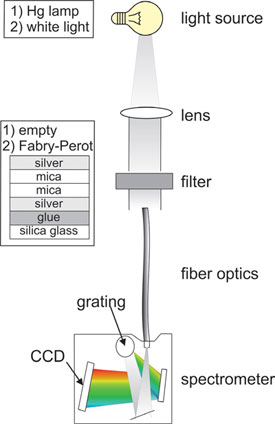
Figure 1 - Setup for interferometry experiments: 1) Rough calibration with mercury lamp. 2) Calibration with an FRF. (Figures reproduced with permission from Ref. 4.)
The key element used is a Fabry-Perot reference filter (FRF), which is typically made of a transparent spacer layer terminated by two highly reflecting mirrors (Figure 1). Broadband illumination with white light yields multiple sharp transmission maxima of similar intensity distributed over the full spectrometer range. The FRF used in the authors’ experiments consisted of two back-silvered mica sheets in direct contact with each other. Mica, which is the spacer layer material, was used due to its excellent cleavage properties and ability to provide large, homogeneous sheets.4
If the thicknesses and refractive indices of all layers of the FRF are precisely known, the transmission spectrum can be calculated and wavelengths can be assigned to the maxima positions on the pixel array. However, the exact spacer layer thickness is, a priori, not known, and can also change during the calibration procedure (e.g., due to thermal expansion). Therefore, it is inevitable to simultaneously determine the exact spacer layer thickness during the calibration procedure. An iterative algorithm that has been developed solves this problem by using two calibration lines of a calibration lamp as anchor lines.4
Experimental accuracy test
Table 1 - Spectrometer specification
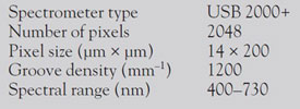
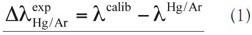
The accuracy of the calibration algorithm using the experimental setup is illustrated in Figure 2. At first, two reference lines (RL3: 435 nm and RL7: 697 nm) of a CAL-2000 Hg/Ar calibration lamp (Ocean Optics, Dunedin, FL) were detected for an initial linear calibration. Next, a halogen lamp illuminated an FRF with a spacer layer thickness of 15.6 μm. The transmitted light was collected by a glass fiber and guided to the spectrometer in order to ensure well-defined incoupling conditions. A USB 2000+ miniature spectrometer from Ocean Optics (Table 1) was used for detection of the spectra. Finally, an eighth-degree polynomial was fitted to the data (wavelengths [λ] at positions [p]). In order to investigate the algorithm’s performance, the accuracy of the calibration method was compared with the accuracy of a conventional calibration. For this, all detected reference lines (RL1–8) were used and a third-degree polynomial was fitted to the data (wavelengths [λ] at positions [p]). The corresponding experimental calibration accuracy was determined by calculating the differences between the wavelengths of the calibration curves and the exact ones known of the mercury/argon lines:
The curvature, κ = λcalib–λlin, of the calibration curve was determined by calculating the wavelength difference between the conventional calibration and the initial linear calibration.
Results
The results of the accuracy test are plotted in Figure 2. The calibration accuracy (top) reflects how well the calibration function reproduces the measured reference wavelengths. The conventional calibration method (triangles) results in a calibration accuracy of 0.4 Å, whereas the new method results in an accuracy of better than 0.2 Å (circles). The curvature κ (Figure 2, center) of the calibration curves reflects the nonlinearity of the light dispersion in the miniature spectrometer. The FRF and calibration lamp spectrum are shown at the bottom of Figure 2.
The new calibration method leads to better calibration accuracies than the conventional method. Further, nonlinearities due to grating distortions or refractive index dispersions in the spacer material can be detected.5
Conclusion
The advantage of the calibration method described here is its ability to calibrate strongly nonlinear miniature spectrometers for spectral ranges in which only a few reference lines are available. The additional calibration peaks from the FRF enable higher-polynomial-order fits, which result in higher calibration accuracies. The new method revealed calibration accuracies below 0.2 Å, which is at least twice as accurate as the conventional calibration. It is important to note that this result was obtained by using a significant amount of calibration lines for the conventional calibration. In ranges where fewer lines are available, the difference would become more profound, revealing the power of the calibration method.
References
- Dorrer, C. J. Opt. Soc. Am. B 1999, 16(7), 1160.
- Fountain, A.W.; Vickers, T.J. et al. Appl. Spectrosc. 1998, 52(3), 462.
- Hamaguchi, H.O. Appl. Spectrosc. Rev. 1988, 24(1–2), 1378.
- Perret, E.; Balmer, T.D. et al. Appl. Spectrosc. 2010, 64, 1139.
- Israelachvili, J.N.; Adams, G.E. J. Chem. Soc. Far. Trans. I 1978, 74, 9758.
Dr. Perret is a Scientist, Paul Scherrer Institut, 5232 Villigen, Switzerland; tel.: +41 3401394; e-mail: [email protected]. Dr. Balmer is a Materials Engineer, ETH Zurich, Zurich, Switzerland. The authors thank Ocean Optics (Dunedin, FL) for its support in testing various spectrometers. This work was funded by the Swiss National Foundation (Bern, Switzerland).