There are indeed statistical issues related to blanks. To set the stage, a discussion of the concept itself will be helpful. On the surface, blanks seem trivial; a blank is a sample (or standard) containing none of the analyte(s). However, simply defining “blank” can be difficult. One of the authors is the Definitions Advisor for the ASTM International Committee D19, which develops test methods (known as Standards) related to the analysis of water. This group has existed for over 75 years, yet the members are still in a lively discussion about what constitutes a blank. Within D19, there is a document devoted solely to definitions that have been developed and approved on a committee-wide basis; the definition of “blank” is being revised to reflect the group’s current thinking about this term. Any test method may define terms specific to that document, and there are many Standard-specific “blank” entries that are preceded by adjectives: 1) calibration blank, 2) field reagent blank, 3) laboratory-fortified blank, 4) laboratory reagent blank, 5) material blank, 6) method blank, 7) reagent blank, and 8) spiked blank. For some of these eight terms, multiple definitions exist among the various applicable Standards. Thus, deciding what is meant by the concept of a blank is difficult and ongoing. (Anyone who is interested in the definition of “blank” is encouraged to participate in D19; please contact Lynn Vanatta for details.)
One of the most significant messages from this multitude of “blank” definitions is that while “absence of the analyte(s)” (or testing to verify its absence) is typically included in the explanation, what other constituents are to be in the sample or standard may vary. Thus, scientists must think carefully about the problem at hand before deciding what constitutes an appropriate blank. In some cases, more than one blank may need to be obtained and tested.
As an illustration, consider the ppt analysis of common anions in deionized water (DIW). Data from a calibration study that included chloride and nitrite have been discussed at length throughout previous installments of this column. The calibration range began with a blank and ended at 200 ppt. What was the appropriate blank for this work? Since all of the standards were prepared in water coming out of a faucet on the DIW line, H2O obtained straight from the tap would be a logical choice. However, standards were prepared by pouring a specific amount of a 500-ppt stock solution into the working-standard bottle and then diluting with DIW (which was collected from the tap into a bottle devoted exclusively to this pure liquid). In the dilution process, the water traveled from its container, through the air, and into the standard bottle (which was then shaken to mix well). As a result, there was ample opportunity for any chloride and nitrite in the air to become incorporated into the standard itself. Indeed, the analysis of a “tap blank” typically shows lower levels of these analytes than does the testing of a “standard-preparation blank” (i.e., water that goes through the entire standard-preparation procedure, except that DIW is added instead of stock standard). Both types of blanks should be tested for this type of study. The tap blank will provide data for deciding if the DIW is clean enough to use for standard preparation. The standard-preparation blank will provide the data to be incorporated into the regression analysis, along with all of the responses from the standards.
From a chemical-analysis point of view, the appropriate blank ideally will contain none of the chemical(s) of interest. It only stands to reason that if all the standards are contaminated with significant, unwanted levels of the analyte(s), then estimating concentrations in ordinary samples will be much more difficult.
It is now time to turn to the statistical side of this topic. From the standpoint of regression, it does not matter whether the blank (and the standards) are contaminated from undesirable sources. The statistical processes of a) choosing an adequate model, b) choosing a fitting technique, then c) evaluating the prediction interval do not depend on the source(s) of the analyte signals.
However, if the scientist wishes to estimate a detection limit (DL) to associate with a calibration (or recovery) curve, then the situation becomes rather dicey. All DL approaches involve blanks, since the inherent goal is to decide if a response is statistically distinguishable from a blank. For example, the 3σ protocol (see Parts 32 and 33, American Laboratory, Nov/Dec 2008 and Mar 2009, respectively) is based on the standard deviation of the responses from blanks (although alternative steps are given if blank data cannot be obtained). The Hubaux-Vos (H-V) detection limit (see Parts 28–30, American Laboratory, Nov/Dec 2007, Feb 2008, and Jun/Jul 2008, respectively) requires that the upper prediction limit (and, therefore, the regression line itself) intersect the y-axis. These lines can always be extrapolated from the lowest standard back to y = 0, but doing so is risky, since there are no data in this region.
Table 1 - Two simulated data sets*
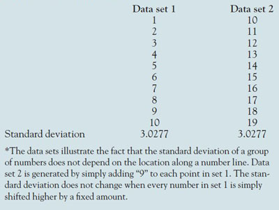
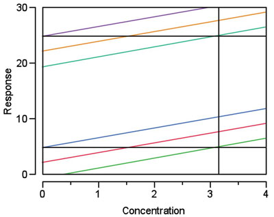
Figure 1 - In this simulated example, calibration (or any regression) lines 1 (red) and 2 (gold) have the same slope. Prediction intervals 1 (darker blue and green) and 2 (purple and lighter blue) have the same width, both intervals are at 95% confidence. The only difference between the two data sets is that the responses in set 2 are each 20 units higher than the responses in set 1. The H-V DL is determined graphically for each set (see black horizontal and vertical reference lines); in each case, the DL is 3.15. In other words, the result is not dependent on the location of the y-intercept.
Thus, unlike being in the world of chemical analysis, operating in the world of detection means that positive blanks are desired, at least from a calculation standpoint! However, the flip side of this DL coin is that the DL (3σ or H-V) is independent of bias (i.e., of the response value at y = 0). At the core, the entire DL concept is based on the precision of the data, not where they are situated in y-vs-x space. Location along a number line does not influence the standard deviation of a set of numbers or the width of a prediction interval. See Table 1 for an example of the former, and Figure 1 for an illustration of the latter.
This “bias-free” characteristic may lead to an unrealistic DL, even in the case of a (more rigorous) H-V calculation. If the precision is tight enough but the blank is positive, the calculated DL may be in the range of (or lower than) the blank’s analyte concentration (which will never be able to be estimated very reliably). From a purely analytical standpoint, the positive blank presents a concentration hurdle that must first be overcome before detection at the calculated DL can be achieved.
This detection-limit dilemma vanishes if calculation of such a statistic is abandoned; instead, every measurement (estimated without extrapolation of the regression line) is reported along with the width of the prediction interval and the confidence level. However, the issue of dealing with positive blanks does not go away. The scientist is still left with deciding if a blank level is low enough for the analytical problem at hand, and what to do if the concentration is deemed too high. How to address this puzzle statistically will be discussed in the next article in this series. Also included will be the option of “forcing zero” during regression (when a blank’s signal is so low that it cannot be distinguished from the baseline noise).
Mr. Coleman is an Applied Statistician, Alcoa Technical Center, MST-C, 100 Technical Dr., Alcoa Center, PA 15069, U.S.A.; e-mail: [email protected]. Ms. Vanatta is an Analytical Chemist, Air Liquide-Balazs™ Analytical Services, 13546 N. Central Expressway, Dallas, TX 75243-1108, U.S.A.; tel.: 972-995-7541; fax: 972-995-3204; e-mail: [email protected].