For the past seven years, this column has chiefly presented basic material related to a single theme: regression analysis of analytical data and the associated uncertainty. After a few introductory articles, the progression has been from design of calibration (or recovery) studies, through regression analysis of the data and evaluation of the prediction interval, to statistically sound approaches to detection and quantitation limits. Now the series will “cycle back” and elaborate on a few specific topics that are related to what has been covered already. Subjects to be discussed will include: 1) deviations, errors, and intervals; 2) blanks; 3) inexact replicates; 4) sampling; and 5) the use of internal standards in electrospray mass spectrometry. This article will discuss the first topic on the list.
In statistics, uncertainty is the name of the game. Without variation in the world, there would be no need for statistical analysis. Because this ideal does not exist and never will exist, scientists need to be able to estimate the variability inherent in data. Several terms are batted about, including: 1) standard deviation (SD), 2) standard error (SE), 3) confidence interval, and 4) prediction interval. These terms are often poorly explained and even incorrectly applied. The situation is enough to make Dorothy, Toto et al. abandon the Yellow Brick Road and Oz, not out of fear of lions, tigers, and bears (oh my!), but out of sheer confusion and exasperation. This article is intended to make some sense out of these concepts, which are interrelated, and to clarify the meaning and usage of each.
The standard deviation is the most basic statistic related to uncertainty. Suppose a chemist analyzed a solution n times to estimate the concentration of a given substance. The SD represents the variability in the data set of n results; the formula is:
SD = [Σ(x – xavg)2 ÷ (n – 1)]1/2
The SD itself is insufficient to describe the population from which the sample was drawn. However, a population can be described by a mean (also calculated from a data set such as the above) and a standard deviation.
The uncertainty in any SD or mean can be calculated, and such an estimate is known as a standard error (SE). The most commonly reported SE is of the mean and is based on the SD for the data set; the formula is:
SEmean = SD ÷ (n)1/2
In general, any time one estimates a statistic, there is an associated standard error that can be calculated. Indeed, the concept applies to the process of regression; not surprisingly, the formulas are more complex.
The basis for regression-related standard errors is the root mean square error (RMSE), which is an estimate of the measurement standard deviation (i.e., inherent variation in the measurement system).
RMSE = [Σ(yi – yfit)2 ÷ dof]1/2
where yi = an individual response in the data set, yfit = the response predicted at that value of x, and dof = the degrees of freedom (for a straight-line model, dof = [n – 2], since 2 dof are “used up” when the slope and the intercept are calculated). The expression (yi – yfit) is the residual for the ith data point (see Part 9 in American Laboratory, Feb 2004, for more information on residuals). The sum of all the squared residuals is cleverly known as the sum of squared residuals (SSR) or residual sum of squares (RSS).
In any regression analysis, a slope and an intercept are estimated. Sometimes, the user is interested in the uncertainties associated with each of these two statistics. RMSE is the starting point for calculating the respective uncertainties, which are standard errors. When multiplied by the appropriate value of Student’s t, these two standard errors respectively become the half-widths of the confidence intervals for the slope and intercept:
SEslope = RMSE ÷ (Sxx)–1/2
SEintercept = RMSE * {(1/n) + [(xavg)2/Sxx]}1/2
where n = the number of data points in the data set, xavg = the average of all the x-values in the data set, Sxx = Σ (xi – xavg)2, and xi = an x-value in the data set.
The next step in the regression-uncertainty process is to ask about the uncertainty associated with the next measurement to be predicted from the regression line. This uncertainty is one of the most important outcomes of a regression analysis. Again, the answer is provided by a standard error, which is based on the SE for the slope and intercept, but has a more complicated formula. As was shown in Part 4 (American Laboratory, Mar 2003), the formula for the half-width of the prediction interval is:
tdof (1 – γ) * (RMSE) * {1 + (1/n) + [(x – xavg)2/Sxx]}1/2
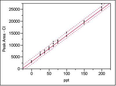
Figure 1 - Regression results for the chloride data (peak area of Cl vs ppt); see text for details.
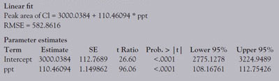
Table 1 - Linear fit and parameter estimates
As with the slope and intercept, the standard error for prediction is everything except Student’s t. (Note: In Part 4, the formula is for calculations in the x-direction; in this article, the width in the y-direction will be considered, meaning that RMSE is not divided by the slope, b.)
As an illustration of the above, consider again the chloride data set presented in the first calibration example in this series of articles (Part 11, American Laboratory, May 2004). Eight replicates of nine standards (blank; 25, 37.5, 50, 62.5, 75, 100, 150, and 200 ppt) were analyzed. Thus, n = 72 (more places than needed for these stats), xavg = 77.7778, and Sxx = 256944.444. A straight-line model with ordinary-least-squares fitting is adequate for these data. From the regression results (see Figure 1 and Table 1; the confidence level is 95%, with α = β = 0.025), RMSE = 582.8616. From the above formulas, the standard errors for the slope, intercept, and prediction (at x = 0) are, respectively:
SEslope = [582.8616/(256944.444)1/2] = 1.149862
SEintercept = 582.8616 * {(1/72) + [(77.7778)2/256944.444]}1/2 = 112.7689
SEregression = (582.8616) * {1 + (1/72) + [(0 – 77.7778)2/256944.444]}1/2 = 593.6703
These calculated values for the standard errors for the slope and intercept match those given in Table 1 (see the “SE” column in the “Parameter estimates” section; “concentration = ppt” represents the slope term). The widths (in the y-direction) of the confidence intervals for the slope and intercept are found by multiplying each standard error by 1.99443711 (≈2), which is the value of Student’s t for the 97.5% level and dof = 70 (i.e. [n – 2] = [72 – 2] = 70). The products are 2.29332801 and 224.909129, respectively. When these values are subtracted and added to the standard-error values, the results are the numbers seen in the “Lower 95%” and “Upper 95%” columns, respectively, in the “Parameter estimates” section of Table 1.
The value for the standard error of prediction is not listed as such in the regression output. However, the 593.6703 is used to generate the prediction interval shown in the plot in Figure 1. To obtain the width (in the y-direction) of this interval at a given value of x (for this example, x = 0), the SE is multiplied by the above value of Student’s t. The result is 1184.038. This value matches the half-width obtained from the graph in Figure 1, if the y-axis is magnified at its intersections with the three curves so that the corresponding y-values can be read. (Note: For another slant on standard deviation versus standard error, see the entertaining, as well as solid and well-written, article, “Maintaining Standards: Differences Between the Standard Deviation and Standard Error, and When to Use Each,” by David L. Streiner, in Can. J. Psychiatry 1996, 41, 498–502.)
Mr. Coleman is an Applied Statistician, Alcoa Technical Center, MST-C, 100 Technical Dr., Alcoa Center, PA 15069, U.S.A.; e-mail: [email protected]. Ms. Vanatta is an Analytical Chemist, Air Liquide-Balazs™ Analytical Services, 13546 N. Central Expressway, Dallas, TX 75243-1108, U.S.A.; tel.: 972-995-7541; fax: 972-995-3204; e-mail: [email protected].