“In almost all cases when dealing with a limit of detection or limit of determination, the primary purpose of determining that limit is to stay away from it.” Thus spoke the late William Horwitz (a chemist with the FDA and AOAC for many years) during a panel discussion on detection limits.1 Indeed, any analyst would prefer to report only measurements that have low uncertainty associated with them. The obvious next step, then, is deciding how far away from the detection limit (DL) the measurement should be in order for the number to be “reportable.” Such discussions fall into the realm of what are often called “quantitation limits” or “reporting limits.” In the opinion of the authors of this column, such limits: 1) are less rigorously calculated and applied than are detection limits and 2) should be abandoned in favor of reporting every measurement (made without extrapolation of the applicable regression curve) along with its prediction interval and associated confidence level. (See Part 26, American Laboratory, Jun/Jul 2007, for an editorial on detection limits.) Such an approach gives the user the statistically sound data he or she needs to make a well-informed decision on the acceptability of the noise level in the measurements. However, other protocols for reporting data are more widely employed. The rest of this article will discuss these procedures and expand on one of them (i.e., the reporting of the number of significant digits).
Unfortunately, the simplest approach (i.e., reporting nothing but the measurement results themselves) is commonplace. Fortunately, with the installation of LIMS in most laboratories, the inclusion of reporting limits has become more common, but how this number has been determined is typically unknown. Thus, the user has no clear estimate of the uncertainty associated with each measurement.
Sometimes, the reporting limit is an extension of the DL, which has been calculated via the 3σ method (see Parts 32 and 33, American Laboratory, Nov/Dec 2008 and Mar 2009, respectively). A common technique is to multiply the DL by 3.18 and use the result as the quantitation or reporting limit. Why 3.18? Answer: If the DL is calculated using seven replicates and α = 0.01, then the DL equals 3.14 times the standard deviation. Hence, multiplying this DL by 3.18 results in a limit that is equal to 10 times the standard deviation. Thus, such a limit is often called “10σ,” and at 10σ, the relative standard deviation is supposedly 10%. However, since important sources of variation (e.g., the uncertainty involved in the regression process) are ignored in the 3σ procedure, these drawbacks apply to the 10σ method as well.
Another protocol is to report the relative uncertainty (ru) associated with the measurement. The formula divides the uncertainty by the measurement (both of which are in concentration units). Such a result is appropriate if the uncertainty estimate is statistically sound, such as is a prediction interval. However, unless the confidence level is also provided, the user still is without some needed information. All too often, though, the ru is based on the same standard deviation that is used in the 10σ approach above.
Another alternative is to report the number of significant digits available. Again, the reader is left without the background information related to the calculation. Frequently, the decision has been based on the number of digits a particular instrument (e.g., an analytical balance) will report. Once again, such an estimate may be completely erroneous, since other aspects of the method have been ignored. However, the basis for reporting significant digits can be statistically sound if prediction-interval half-widths are the source of the uncertainties. The concept allows for fractions of a significant digit and will be explained in the remainder of this article.
At the outset, a fundamental truth is crucial and must be kept in mind throughout the discussion. The reality is that the number of significant digits depends solely on the magnitude of the uncertainty associated with the measurement.
To understand this fact, consider the measurement 1.0. If the information content is such that this number contains precisely two significant digits, then the associated uncertainty is ±0.05. In other words, the uncertainty interval is 0.95 to 1.05. Within that range, the measurement will always round to 1.0. As soon as the ±uncertainty exceeds this range, then a measurement of, e.g., 1.051 is possible; such a number will round to 1.1, so the second significant digit is lost. Similarly, 0.949 is possible. This number rounds to 0.9; again, the second significant digit is lost.
The interval ±0.05 can be expressed by the one-sided uncertainty: 0.5 * 10–1. Note that the exponent is one less than the number of significant digits (ignoring the negative sign). This relationship holds in general. The ±uncertainty (u) can be stated as 0.5 * 10–(d–1), where d is the number of significant digits. Or:
u = 0.5 * 10(1–d)
Calculation of d in terms of u requires the use of logarithms (base 10):
log (u) = log (0.5) + log (101) + log (10–d) = log (0.5) + 1 – d
d = log (0.5) + 1 – log (u)
(Remember that the log of n numbers that are multiplied together is the same as the sum of the logs of the n individual numbers.)
Log (0.5) is ca. –0.3, so:
d ≈ 0.7 – log (u)
Thus, if u becomes too large, d will become negative.
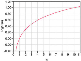
Figure 1 - Relationship between a number and its logarithm. Note that the plot is not linear in n. Since the number of significant digits (d) is based on logarithms, d will not be linearly related to the uncertainty (u), either.
Also, remember that the logarithm function is not linear. Figure 1 shows the relationship between the two variables. Thus, d will not be related linearly to the uncertainty.
The expression can be written in terms of relative uncertainty, since ru = u/c, where c is the concentration. Thus,
d = log (0.5) + 1 – log (ru * c), or
d = log (0.5) + 1 – log (ru) – log (c)
The same logarithm realities also apply to this version of the relationship.
In the next installment, the implications of the above formulas will be explored in more detail.
Reference
- Horwitz, W. In Detection in Analytical Chemistry. Importance, Theory, and Practice; Currie, L.A., ed.; ACS Symposium Series 361, American Chemical Society: Washington, DC, 1988; p 310.
Mr. Coleman is an Applied Statistician, Alcoa Technical Center, MST-C, 100 Technical Dr., Alcoa Center, PA 15069, U.S.A.; e-mail: [email protected]. Ms. Vanatta is an Analytical Chemist, Air Liquide-Balazs™ Analytical Services, 13546 N. Central Expressway, Dallas, TX 75243-1108, U.S.A.; tel.: 972-995-7541; fax: 972-995-3204; e-mail: [email protected].