The subject of detection limits (DLs) is a controversial one, generating many questions and almost endless debate. To summarize this column’s treatment of DLs, this article will present a series of questions (which the authors have often been asked) and answers.
How does one define “detection limits”?
This term produces almost as many definitions as there are people who deal with this topic. In general, practitioners tend to divide into two camps: 1) the probability of false negatives (i.e., β) should be controlled when calculating a DL, and 2) only the probability of false positives (i.e., α) needs to be addressed. Thus, it is difficult to craft a definition that satisfies everyone.
However, the concepts that are inherent in Receiver Operating Characteristic (ROC) curves (see Parts 27 and 31, American Laboratory, Sep 2007 and Sep 2008, respectively), and in the work of Hubaux and Vos (see Parts 28 and 29, American Laboratory, Nov/Dec 2007 and Feb 2008, respectively) can be used to derive a fairly generic definition of a detection limit.
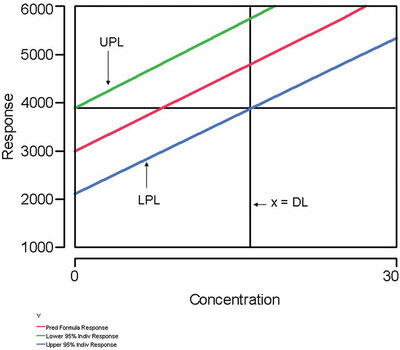
Figure 1 - This plot illustrates a generic definition of a detection limit. See the first question/answer in the text for details.
“A detection limit (in concentration units) is any combination of α, β, and concentration that satisfies the following relationship, which references Figure 1: The response corresponding to the intersection of the upper prediction limit (UPL) with the x = 0 line is the same as the response corresponding to the intersection of the lower prediction limit (LPL) with the x = DL line.”
Since a detection limit can be described mathematically by one equation in three unknowns (which are α, β, and the DL), the above definition allows the user to assign values to any two of the three variables. By the rules of algebra, the value of the third and final variable is determined by the equation, which now has become a single-variable equality. If the user is not concerned with β, then the definition allows for such a situation. However, the false-negative probability still exists.
Why do some detection limits result in having one of the prediction limits “cross” over the regression line?
This situation may occur if a detection limit is driven lower and lower. To compensate for the low value of the DL variable, the value of either α or β must rise. If either probability exceeds 50%, then the corresponding prediction limit will “cross” the regression line (see Part 32, American Laboratory, Nov/Dec 2008).
How should the user proceed if a “crossover” situation occurs?
In such situations, the DL should not be considered to be valid. No longer can a predicted concentration be reported as “plus or minus an uncertainty.”
If a specific low DL is required to meet requirements for the analytical method, then the user has a few options. First, a new calibration (or recovery) study can be designed and conducted, whereby only very low concentrations are used. Such an approach may result in a lower (but still statistically sound) DL. Second, the power of averaging can be invoked. Using averages will decrease the standard deviation by a factor of (1/√n), where n is the number of data points used to calculate the average. Note, though, that if averages are used to calculate the DL, then the same averaging process must be used when sample data are analyzed.
How does one calculate “the” detection limit for a given analytical method?
The concept of “the” detection limit does not exist! First and foremost, any DL is tied inextricably to the data set that was used for the calculation. Also, the value of the limit depends inherently on the values of α and β (always remember that the world of detection is described by one equation in the three unknowns of α, β, and the DL).
Shouldn’t the user design and conduct a “pristine” study to try to discover the lowest DL that is possible?
While there is nothing wrong with conducting such a study, doing so is an academic exercise if the design will not be applied to real-world samples. It cannot be overemphasized that any DL is linked totally to the data set that generated the value. Any “tricks” used to generate a very low DL must be used when samples are analyzed, if the low DL is to be associated with the reported sample results. Furthermore, a DL that is calculated using standards in pure solvents cannot be associated automatically with samples whose results are subject to matrix effects.
Are there ways to decrease a statistically sound DL, short of purchasing a more sensitive and less noisy analytical instrument?
As mentioned earlier, the power of averaging can be utilized. Also, the values of α and β can be raised, although neither realistically should rise to more than about 10%.
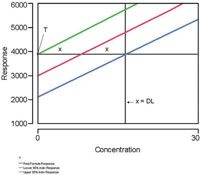
Figure 2 - This graph illustrates why the uncertainty at a Hubaux-Vos (H-V) detection limit (DL) is approximately ±50%. The uncertainty is approximately (x/2x), which is about 0.50. “T” is the threshold, the response below which a measurement cannot be distinguished from zero.
What is the relative uncertainty associated with a reported measurement that is at the DL (assuming that α and β have been controlled and have been set equal to each other)?
In these situations, a Hubaux-Vos (H-V) DL has been calculated. For these cases, the uncertainty is always approximately ±50% (“approximately” because the percentage is based on the assumption that the prediction-interval curves are nearly straight lines and parallel to each other). Figure 2 illustrates this reality. Each uncertainty is x, while the value of the H-V DL can be expressed as 2x. The relative uncertainty is (x/2x), or 0.50.
What should the user do if the calculated H-V DL is lower than the lowest non-zero standard in the calibration design?
If the DL will be used for reporting purposes, then the lowest concentration used should also be reported to the customer. However, if time and resources allow, a new study should be conducted, this time including even lower concentrations in the design. In other words, the analytical method can handle low levels even better than the user first imagined!
Isn’t it sufficient to analyze a multilevel calibration (or recovery) design once and calculate a H-V DL from those data?
If the user desires a low (and statistically sound) DL, this shortcut should not be employed. First, without replicates, the standard deviation cannot be modeled. Thus, ordinary least squares (OLS) must be the fitting technique. However, if weighted least squares is actually what is needed, then the user has robbed himself or herself of the opportunity to work with a prediction interval that flares, almost always with increasing concentration. If the flaring is significant, then the prediction-interval width will be significantly less at low concentrations (i.e., in the DL range) than it is when OLS is applied.
Second, the prediction interval may be quite wide if only a few data points are available. Remember that several terms in the prediction-interval equation decrease as n increases.
How can a laboratory conduct the recommended calibration (or recovery) study (i.e., multiple levels and multiple concentrations) if the instrument is used continuously for sample analyses?
The solution to this dilemma lies in the analysis of check standards, which are tested routinely in virtually all analytical laboratories these days. Most times, a single concentration is selected and analyzed each time the standard operating procedure requires such a check. However, the user can be creative and vary the concentration each time, using (in random order) the concentrations that are in the study design. Over the course of several days, the desired number of replicates can be tested. This approach inherently achieves another goal of such a study (i.e., to capture typical day-to-day variability in the analytical method). In the end, the user will have all of the desired data and will not have had to analyze a single extra standard or sample!
Mr. Coleman is an Applied Statistician, Alcoa Technical Center, MST-C, 100 Technical Dr., Alcoa Center, PA 15069, U.S.A.; e-mail: [email protected]. Ms. Vanatta is an Analytical Chemist, Air Liquide-Balazs™ Analytical Services, 13546 N. Central Expressway, Dallas, TX 75243-1108, U.S.A.; tel.: 972-995-7541; fax: 972-995-3204; e-mail: [email protected].