In the last installment (Part 32, American Laboratory, Nov/Dec 2008) of this series, three detection limits (DLs) were calculated (via the 3-Sigma [3σ] approach, where α is set to be 0.01) for a chloride data set. These DLs were 9.3, 16.2, and 14.2 ppt, calculated using data from blanks, 25-ppt standards, and 37.5-ppt standards, respectively. The associated value of β was also determined for each DL: 0.748, 0.263, and 0.397, respectively. These calculations were made to emphasize the importance of thinking about β when living in the world of DLs. Although the false-negative rate can be ignored (and often is), it always exists. If not controlled, β may very well be at an unacceptably high level.
If asked, most people would like to keep the DL process simple and to have the confidence level be high. These desires mean that α and β: 1) should be equal to each other and 2) should be low, thereby meaning the confidence level should be high. While “high enough confidence” depends on the application, the lowest confidence level that typically is tolerated is 80% (meaning that the simple case is α = β = 10% or 0.1). For the data set used in Part 32, such a restriction results in a DL of 14.0 ppt. (Remember that once α and β have been selected, the third/final variable in the DL equation is the DL itself, and it cannot be chosen by the user.)
The above result is in the ballpark of the three DLs given in the first paragraph. Thus, the following question arises: If a given value of a detection limit is desired, then what would be the associated α and β, given the stipulation that the two probabilities must be the same?
Once again, the answer begins with Eq. (13) from Part 31 (American Laboratory, Sept 2008):
[(b ∗ xD)/(RMSE ∗ RxD)] – [(t1-α ∗ R0)/RxD] = t1-β
In this instance, though, since α and β are the same, the references to either can be replaced with the generic variable, γ. Making that replacement and combining the t terms on the right side of the equation results in:
[(b ∗ xD)/(RMSE ∗ RxD)] = t1-γ + [(t1-γ ∗ R0)/RxD]
Or,
[(b ∗ xD)/(RMSE ∗ RxD)] = [(RxD ∗ t1-γ)/RxD] + [(t1-γ ∗ R0)/RxD]
Combining t terms results in:
[(b ∗ xD)/(RMSE ∗ RxD)] = [(t1-γ) ∗ (RxD + R0)]/RxD
The t term can be isolated on the right side of the equation:
[(b ∗ xD)/(RMSE ∗ RxD)] ∗ [RxD/(RxD + R0)] = (t1-γ)
Or,
(b ∗ xD)/[RMSE ∗ (RxD + R0)] = (t1-γ)
For any chosen DL, this final equation will return the Student’s t value for (1 – γ) such that α and β are the same. The t distributions for each value will result in the value of (1 – γ) itself, from which α can be extracted.
As stated in paragraph one, the DLs calculated in Part 32 were 9.3, 16.2, and 14.2 ppt. Using the above equation and determining the associated t distributions reveals that the γ values are 0.195, 0.068, and 0.095, respectively. Thus, the overall confidence levels (1 – 2γ) are 0.610, 0.864, and 0.810. As always, only the user(s) can decide if any of the confidence levels calculated here are acceptable for the application at hand.
It may be tempting to think that the DL can be pushed ever lower, if the confidence level is assumed to be unimportant. However, there is a limit to this process. As was mentioned in Part 32, once a probability reaches 0.5, the associated value of Student’s t is zero. As a consequence, the formula for the prediction limit also goes to zero. Thus, if α = β = 0.5, then the prediction interval ceases to exist. Therefore, the chance line has been reached; no matter what value of α is chosen, the associated value of β will be such that the sum of the two is 100%. In other words, the confidence level is zero; there is then no point in analyzing samples, since one might as well draw result values out of a hat!
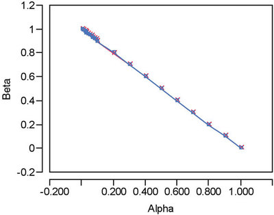
Figure 1 - Overlay of the ROC curve for a chloride DL of 0.014 ppt with the chance line. On this scale, the two lines are indistinguishable.
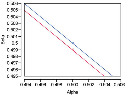
Figure 2 - Magnification of a portion of the overlay shown in Figure 1. Only on this scale can the very slight offset of the two curves be seen.
With the chloride data that are being used here, what is the lowest DL that will have a positive, non-zero confidence level associated with it (however small and intolerable it may be)? The simplest path to the answer is to approximate the DL graphically. If the confidence level is dropped to the “nearly zero” value of 0.001 and α is equal to β, then the resulting DL is 0.014 ppt. The Receiver Operating Characteristic (ROC) plot for this situation is given in Figure 1. Also included is the chance line, although on this scale, the two lines are indistinguishable. Only by zooming in can the slight offset be detected (see Figure 2). Thus, any significant reduction in the DL from 0.014 ppt is meaningless (as is 0.014 ppt or any low-confidence-level DL, for all practical purposes).
One further comment should be made about working with a situation where either α or β is greater than 0.5 (i.e., where one of the prediction limits has “crossed over” the regression line). In the real world of reporting results along with a prediction interval, one of the concepts behind such an interval has now been violated. One must be able to report the result plus an uncertainty as well as minus an uncertainty. Thus, in these high-α or high-β cases, the “crossed-over” prediction limit is invalid and cannot be interpreted. It also should be added that both α and β cannot be greater than 0.5, since then the sum of the two would be greater than 1.0 (or 100%), and such a situation is impossible statistically.
Mr. Coleman is an Applied Statistician, Alcoa Technical Center, MST-C, 100 Technical Dr., Alcoa Center, PA 15069, U.S.A.; e-mail: [email protected]. Ms. Vanatta is an Analytical Chemist, Air Liquide-Balazs™ Analytical Services, 13546 N. Central Expressway, Dallas, TX 75243-1108, U.S.A.; tel.: 972-995-7541; fax: 972-995-3204; e-mail: [email protected].