In Part 29 (American Laboratory, Feb 2008), Hubaux-Vos detection limits (H-V DLs) were explained and an illustration was given. The article ended with two new graphs for the reader to investigate on his or her own. The plots (see Figures 1 and 2, each of which includes the construction of the H-V DL) were both based on the same regression line as was used in the Part 29 illustration. However, in each “homework assignment,” the prediction limits were a different distance from the regression line. The goal was to decide: 1) what had happened to α, β, and the H-V DL; and 2) why each change had occurred.
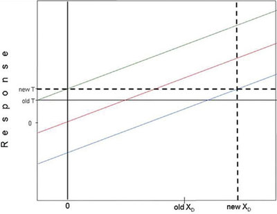
Figure 1 - Solution to first “homework” problem. See text for details.
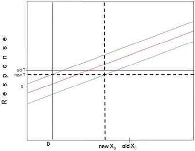
Figure 2 - Solution to second “homework” problem. See text for details.
The first part of this installment will answer these questions. The remainder of the article will apply the H-V concepts to two real-world data sets.
Before the two figures are diagnosed, it is important to emphasize the directional effects of α and β on the width of the prediction interval. Recall that α and β each represent a probability of being wrong. In the case of α, its value is the probability of being wrong when a blank is being analyzed (i.e., of having a false positive, FP). In the case of β, its value is the probability of being wrong when the analyte of interest is present (i.e., of having a false negative, FN). For both α and β, the higher the value, the more risk the user is willing to take of being wrong. The overall confidence level for the prediction interval is [1 – (α + β)], meaning that the higher the values of α and β, the lower the confidence level.
The prediction limits represent the boundaries set by the chosen values of α and β. Relative to the regression line, the position of the upper limit is influenced by α, while the location of the lower limit is influenced by β. The width of this interval represents the confidence level. Any values that fall outside either limit are, so to speak, part of the acceptable-risk-factor population.
If either α or β increases (or both increase), then the risk of being wrong has been allowed to increase. Thus, more data points are allowed to fall outside of the prediction-interval envelope and its width decreases. If either α or β decreases (or both decrease), then the risk of being incorrect has been allowed to drop. As a result, the effect on the prediction interval is the opposite (i.e., the width increases), since relatively fewer data points should be outside the envelope.
The situation is analogous to driving down a road. If someone is driving in western Texas, where the terrain is quite flat for miles, then it doesn’t much matter if the car goes off the road (assuming the ditches are not too deep). Hence, the pavement can be quite narrow, since a “false location” is fairly insignificant. However, if the person is in the Rocky Mountains, then staying on the road is often a matter of life or death. In such situations, a wide road is much preferred (although, unfortunately, often not available!), since the consequences of a misstep are severe.
The above discussion must be kept in mind when evaluating Figures 1 and 2. In the first case, the prediction limits are farther apart than they were in the original illustration in Part 29. Thus, the user wants to be more certain that the data points remain inside the envelope. Since the confidence level has risen, α or β or both must have decreased. Here, both limits have moved away from the regression line, so both α and β have decreased. Figure 1 also shows the graphic determination of the H-V DL, which depends on the values of α and β, and thus on the width of the prediction interval. The DL has increased, as it must. Such an occurrence makes sense. If there are to be fewer FPs for blanks and fewer FNs for low-level standards (or samples), then the detection limit must rise.
For Figure 2, both limits are closer together than they were originally. Thus, fewer data points fall inside the envelope. In other words, the confidence level has been allowed to drop. Thus, α and β have both increased. Because the probabilities of FPs and FNs can be higher now, the H-V DL is lower than it was in the Part 29 illustration.
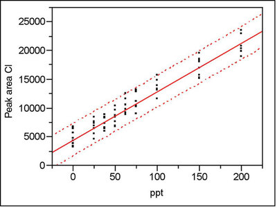
Figure 3 - Calibration plot (with prediction interval) for chloride in deionized water. Confidence level is 95% (α = β = 2.5%).
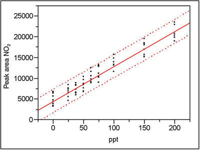
Figure 4 - Calibration plot (with prediction interval) for nitrite in deionized water. Confidence level is 95% (α = β = 2.5%).
To apply the above concepts to real-world data, recall Parts 11 (American Laboratory, May 2004) and 12 (American Laboratory, Jul 2004) in this series of columns. In both articles, the data (for chloride and nitrite, respectively) were from a calibration study involving trace levels of anions in deionized water. The calibration design had nine concentrations (a blank and eight non-zero levels ranging from 25 to 200 ppt). Figures 3 and 4 show the calibration plots and their associated prediction intervals (at 95% confidence). Both plots have the same scale on the x- and y-axes. The y-axis is in units of peak area; the x-axis is in concentration units of parts-per-trillion (weight/weight) or ppt. For these values of α and β, what is the H-V DL for each analyte?
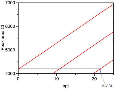
Figure 5 - Same as Figure 3, with the lower-left corner enlarged. Graphic determination of the H-V DL (~22 ppt, with α = β = 2.5%) is shown.
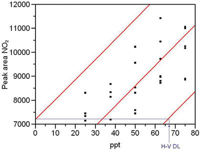
Figure 6 - Same as Figure 4, with the lower-left corner enlarged. Graphic determination of the H-V DL (~67 ppt, with α = β = 2.5%) is shown.
To determine these detection limits graphically, it is helpful to enlarge the lower left-hand portion of each plot (see Figures 5 and 6 for chloride and nitrite, respectively). In each graph, the necessary lines have been constructed to determine the H-V DL. This detection limit is ~22 ppt for chloride and ~67 ppt for nitrite.
Why is there a threefold difference between the two DLs? Although the average peak area for a given concentration is approximately the same for the two analytes, the prediction interval is wider for nitrite than for chloride. In this case, the increased width is not due to a decrease in α or β (remember that the confidence level for both is 95%). Recall from Part 4 (American Laboratory, Mar 2003) that the width of the prediction interval depends on several variables, an important one of which is the noise in the data (typically quantified by RMSE, root mean square error). In Figures 3 and 4, note that at any given concentration, there is more scatter in the nitrite data than there is in the chloride responses. Thus, the RMSEs are different (583 for chloride and 1378 for nitrite) and the widths of the prediction intervals are different as well.
The reader may wonder why the ratio of the H-V DLs (in concentration units) is NO2/Cl ≈ 3/1, while the ratio of the RMSEs is NO2/Cl = 1378/583 ≈ 2.4. (Since the calibration design, α, and β are the same for both analytes, the only difference in the formula for the prediction limits is RMSE, which acts solely as a multiplier.) Recall from Part 4 (American Laboratory, Mar 2003) that during the regression process, the prediction limits are determined in the y-direction. If, at each DL concentration, the width of the prediction interval is measured in response units, the ratio is the same as is that of the RMSEs. Since the transformation (via the regression line) from y-units to x-units is not a simple scaling process, the ratio in x-units is different from the ratio in y-units.
Mr. Coleman is an Applied Statistician, Alcoa Technical Center, MST-C, 100 Technical Dr., Alcoa Center, PA 15069, U.S.A.; e-mail: [email protected]. Ms. Vanatta is an Analytical Chemist, Air Liquide-Balazs™ Analytical Services, 13546 N. Central Expressway, Dallas, TX 75243-1108, U.S.A.; tel.: 972-995-7541; fax: 972-995-3204; e-mail: [email protected].