Part 28 (American Laboratory, Nov/Dec 2007) laid the framework for discussing detection limits. The relationship among the detection limit (DL), the probability of false positives (α), and the probability of false negatives (β) was detailed. The article ended by showing a plot that began to tie these three variables to calibration curves. That diagram is repeated in Figure 1, with the addition of a vertical line from the lower prediction limit to x = xD. This graph is crucial to understanding detection limits. The message from the figure is that α, β, and the DL are related graphically via the combined lines of (y = T, the threshold response) and of (x = xD). For a given combination of α and β, the associated detection limit is xD. This concentration is the lowest concentration that can be detected (i.e., the user is working at the threshold response of T, with its associated value of α; T is the lowest response that can be distinguished from zero) and still control β at the value represented by the lower prediction limit. No other concentration will allow for the desired control of both α and β for a single analytical measurement.
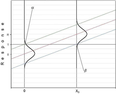
Figure 1 - Combined graph showing: 1) the distribution of responses obtained from analyzing, in replicate, a blank sample and a low-level sample of concentration r, and 2) the calibration curve with its associated prediction interval. The x-axis has units of frequency of occurrence (for the Normal curves) and of concentration (for the calibration curve and prediction interval). On the x-axis, the value of the H-V DL (xD) is also shown.
To understand the above “message” more clearly, recall that (relative to the calibration curve itself) the location of the upper prediction limit (UPL) is influenced by the value of α; the location of the lower prediction limit (LPL) is tied to the value chosen for β. For blanks, the upper end of the distribution curve for responses will intersect the UPL such that the area above this limit is α. Thus, when measuring a blank, the likelihood that the response will exceed T is α. For any standard with response R, the distribution curve will always intersect the LPL such that the area below this limit is β. [Keep in mind that calibration (and all regression) curves and associated prediction intervals are generated in the x-to-y direction. In other words, known values of x are tested (analyzed) and responses (y values) are generated.]
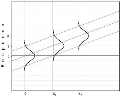
Figure 2 - Plot showing a candidate DL that is lower than the H-V DL shown in Figure 1.
Why is a value such as x1 (see Figure 2) not a candidate for the DL (given the same chosen values of α and β)? As always, a β proportion of this concentration’s distribution lies below the LPL. However, the corresponding response value is well below T, and thus is indistinguishable from zero (i.e., cannot be detected at all).
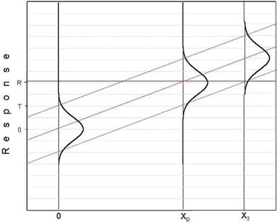
Figure 3 - Plot showing a candidate DL that is higher than the H-V DL shown in Figure 1.
A concentration value above xD (e.g., x2 in Figure 3) is not a DL candidate since the associated response is above the threshold and would result in a false-positive rate (i.e., α) lower than what has been chosen. Besides, in calculating a DL, the goal is to find the lowest possible value that will satisfy the starting conditions!
This determination of the DL from the prediction intervals was the work of two scientists named Hubaux and Vos. They published their theoretical paper in Analytical Chemistry in 1970.1 Thus, DLs that quote associated values of α and β are called Hubaux-Vos (H-V) detection limits.
From a practical standpoint, the user of a calibration curve can easily estimate the H-V DL using most statistical-software packages. Once the curve and prediction limits have been plotted, the cursor can be changed to cross-hairs, which automatically show the associated x- and y-values for any point on a graph. The horizontal line is fixed at y = T, and the vertical line is moved until it intersects the LPL. The x-value at that intersection (i.e, the H-V DL, in concentration units) is then read.
While α is typically set to be the same value as β, such an equality is not mandatory. The result of an inequality will be that the UPL and LPL will no longer be equidistant from the calibration line (or any regression line). (In addition, the measurement uncertainty will no longer be reported as plus or minus a single value; the upper uncertainty limit will be a different distance from the regression line than will be the lower uncertainty limit.) However, the H-V DL can still be determined graphically by the same procedure outlined above.
Figure 4 - Same calibration curve as shown in Figure 1. However, the prediction limits are farther apart than in the original graph. The original DL (xD) and its distribution are shown for reference.
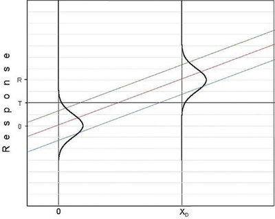
Figure 5 - Same calibration curve as shown in Figure 1. However, the prediction limits are closer together than in the original graph. The original DL (xD) and its distribution are shown for reference.
As has been mentioned several times in the past two articles in this series, for a given data set, α, β, and the DL cannot all be held to user-selected low values. For a given DL, the only way to lower α and β simultaneously is to obtain a better data set (i.e., a set with less noise). In other words, the user will have to improve the analytical procedure. However, such an alternative typically involves the expenditure of money (e.g., paying more for method development and analysis time, and/or for new instrumentation). As in the rest of life, there is no free lunch in the statistical world, either!
It must be emphasized that if α or β (or both) are changed, then the detection limit will change, too. The DL must move, since the positions of the UPL and LPL (which are influenced by α and β, respectively) will move. As a “homework” assignment for the reader, Figures 4 and 5 are presented. Both show the same calibration curve as is in Figure 1. However, in Figure 4, the prediction limits are farther apart than they are in Figure 1; in Figure 5, the limits are closer together. For each plot, the questions to be answered are: 1) Did the value of α increase or decrease? 2) Did the value of β increase or decrease? 3) Did the value of the H-V DL increase or decrease? [The original DL (xD) and its distribution are shown for reference.] 4) For the previous three questions, why did the increase or decrease occur (based on the positions of the prediction limits)?
Reference
- Hubaux, A.; Vos, G. Decision and detection limits for linear calibration curves. Anal. Chem. 1970, 42, 849–55.
Mr. Coleman is an Applied Statistician, Alcoa Technical Center, MST-C, 100 Technical Dr., Alcoa Center, PA 15069, U.S.A.; e-mail: [email protected]. Ms. Vanatta is an Analytical Chemist, Air Liquide-Balazs™ Analytical Services, 13546 N. Central Expressway, Dallas, TX 75243-1108, U.S.A.; tel.: 972-995-7541; fax: 972-995-3204; e-mail: [email protected].