A number of methods are used to measure the viscosity of fluids. These are typically based on one of three phenomena—a moving surface in contact with a fluid, an object moving through a fluid, and fluid flowing through a resistive component. These phenomena utilize three major viscometers in the industry, i.e., a rotating viscometer, a falling-ball viscometer, and a capillary viscometer. The falling ball viscometer typically measures the viscosity of Newtonian liquids and gases. The method applies Newton’s law of motion under force balance on a falling sphere ball when it reaches a terminal velocity. In Newton’s law of motion for a falling ball, there exist buoyancy force, weight force, and drag force, and these three forces reach a net force of zero. The drag force can be obtained from Stokes’ law, which is valid in Reynolds numbers less than 1.1–3
The falling ball viscometer is well-suited for measuring the viscosity of a fluid, and the method has been stated in international standards.4,5 In the international standards, the method differs from the principle described in Refs. 1–3. The standards describe an inclined-tube method in which the tube for the falling ball was inclined at 10° to the vertical. Moreover, six balls were used with different diameters for various dynamic viscosity measurement ranges, and a suitable ball can be selected when the fall times of the ball are not lower than the minimum fall times recorded during a testing procedure. The rolling and sliding movement of the ball through the sample liquid are at times in an inclined cylindrical measuring tube. The sample viscosity correlates with the time required by the ball to drop a specific distance, and the test results are given as dynamic viscosity.
Brizard et al.6 developed an absolute falling ball viscometer and made it possible to cover a wide range of viscosities while maintaining a weak uncertainty. This method considered the effect of edge, inertia, etc., and corrected the measurement result to reach a relative uncertainty on the order of 0.001. Capper Ltd. (Stoke-on-Trent, Staffordshire, U.K.) devised an improved instrument (patent no. GB1491865) for the measurement of viscosity. The instrument applied the first and second coils at different known positions around the falling tube to record the falling time in order to avoid human error. Nevertheless, the apparatus is limited in application for a stainless steel ball.
Although the falling ball method has been well developed and is stated in the international standards, it is somewhat inconvenient to operate this type of viscometer. For example, the viscometer requires six different diameter balls to measure a varying range of viscosities, and the user must run tests to select a suitable ball. Moreover, it is difficult to determine where the falling ball arrives at the terminal velocity, i.e., whether the distance between the beginning record line and the starting fall position is sufficient. Additionally, the inclined-tube viscometer is 10° to the vertical; thus the falling ball is not just falling down but is also rolling down. This phenomenon is different from the conditions in the derivation of the falling ball method.1–3 Therefore, the purpose of this study was to develop a new method based on the traditional falling ball method, while deriving a dynamic equation for describing falling ball behavior in a vertical tube. Because this type of viscometer is vertical to the ground, it will be referred to here as a vertical falling ball viscometer.
Analysis
A falling ball viscometer has a sphere ball that falls down along a tube containing the sample liquid to be measured, and this tube is surrounded concentrically by a tubular jacket for thermal control. The previous theory used Newton’s law of motion for describing the falling ball reaching a terminal velocity; thus, the net force of gravity, buoyancy, and drag is zero:
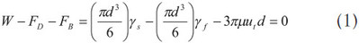
The drag force is expressed in the third term on the right side of the equal sign according to Stokes’ law, which is valid in Ref. 1. Eq. (1) can be easily expressed in the following form:
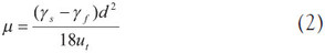
Where γ is the specific weight, d is the diameter of the sphere, and ut is the terminal velocity. The subscripts s and f represent the sphere and fluid, respectively. Eq. (2) can be simplified to the following form and is the same as that claimed in the standard4:
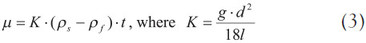
Where l is the falling length and t is the time passing the length of l.
When the material properties, geometric properties, and falling time are known, the viscosity can be obtained from Eq. (2) or (3). In the standards,4,5 the coefficient of K must be estimated by measuring a reference liquid with a known viscosity. Then, the viscosity of an unknown liquid can easily be calculated in Eq. (3), when the falling time is known.
The present study focuses on the motion of a sphere ball falling from the beginning to the end; thus it exists in the acceleration term in Newton’s law of motion:

Eq. (4) can be expressed in the following form after substituting the volume expression of a sphere:
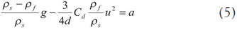
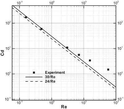
Figure 1 - Drag coefficient versus Reynolds number of a sphere moving in liquid.
The drag coefficient of a sphere, Cd, has been tested and the results plotted against the Reynolds number.7–9 Assuming the inertia terms in the equation of motion of a viscous fluid can be disregarded in favor of the terms involving the viscosity, Stokes’ law states the drag coefficient as the form, Cd = 24/Re. Figure 1 depicts the drag coefficient versus Reynolds number with the experimental results and two curve-fitting lines. The solid square, dashed line, and continuous line represent the experimental data, the line of Stokes’ expression, and the line of Cd = 30/Re, respectively. It is clear that the continuous line is preferable to the dashed line based on the matching of the solid square when the Reynolds number is less than 5. Therefore, the study selects the relationship between the drag coefficient and the Reynolds number as follows:
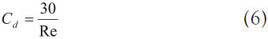
The study substitutes Eq. (6) for Eq. (5), and the following form is obtained:
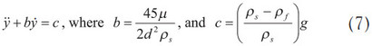
The initial conditions were:

The exact expression of Eq. (7) can be solved as follows:
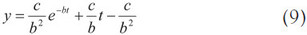
In Eq. (9) it is difficult to find an explicit expression for the viscosity through the known parameters and the falling time, because the viscosity is implicit in the equation. Therefore, the study designed a numerical program to pursue the viscosity in Eq. (9) by the iteration scheme. The process of the numerical program is: 1) Set the parameters of material and geometry; 2) calculate the distance of y from Eq. (9) by guessing the viscosity; 3) check the relative error between the calculated distance and the falling distance, and correct the guessed value of viscosity; 4) repeat steps 2 and 3 until the relative error of distance is below the convergence criteria; 5) check the Reynolds number to see if it is less than 5. If it is not, the result must be discarded and the ball replaced with another of different density or diameter.