The previous article (American Laboratory, Apr 2011)
ended with an unsolved problem: how to implement
a pass-fail method if the blank matrix contains a non-negligible
amount of the analyte. This installment will
address the above situation.
The best way to proceed would be to locate a simulated or synthetic
matrix that is as similar as possible to the material at
hand. Then the analyst would have the “true blank” needed for
applying the above protocol. An example would be drinking-water. Calibration and recovery curves for ionic environmental
contaminants could be studied by preparing (in, e.g., deionized
or reagent-grade water) a solution containing typical drinking water
levels of chloride, carbonate, nitrate, and sulfate. Such
a simulation would not, by construction, contain any of the
analyte(s) of interest.
Another route would be to use a “recipe” adopted by a consensus-based
organization. The D19 Water Committee of ASTM International
(formerly known as American Society for Testing and Materials)
has developed both substitute ocean water and substitute
waste water. Such matrices may provide an acceptable substitute
for some methods.
If a simulated matrix is not feasible for whatever reason, then the
approach is more involved and using regression is almost inevitable.
A suggested path is the following and assumes that the blank
level is thought to be roughly at or below the spec level. The first goal
is obtaining as reliable an estimate as possible of the amount of analyte
in the blank.
Step 1—Estimate blank’s level via a calibration curve
A calibration curve (in pure solvent) (see earlier installments of
this column for details on calibration) should be obtained in the
concentration range of interest. This plot can then be used to
calculate a rough estimate of the blank’s analyte concentration.
(The qualifier of “rough” is used because no information is available
about the analyte’s recovery in matrix.)
Step 2—Conduct a spiking study to assess recovery
To check the rough estimate (and get a handle on recovery),
a spiking study (in the matrix) should be conducted, where
the top concentration is at least twice the rough estimate. A
minimum of three concentrations should be chosen between
the rough estimate and the doubled amount. If possible, each
concentration should be analyzed five times. A recovery curve
(see Parts 20 and 21, American Laboratory, Feb 2006 and Apr
2006, respectively, for a discussion of recovery curves) then can
be generated from the pure-solvent calibration curve (assuming
the concentration range is similar to that in the spiking work).
If the recovery is “close” to 100%, then the rough estimate probably
is a reasonable one.
Especially if the recovery is “well away” from 100%, the blank’s estimate
can be checked by comparing the response for the blank itself
with the response from the “twice-the-estimate” spike. If the higher
number is ca. twice the lower, then the estimate is probably reasonable.
Step 3—Utilize standard addition as a final check
If all is “OK” so far, then standard addition could be employed
as a final check on the blank’s estimate. (As has been mentioned
previously, standard addition, though often used as the only
alternative, has statistical drawbacks; for details, see American
Laboratory, Part 21.)
If the recovery curve: 1) is linear, 2) has a prediction interval with
an acceptable half-width, and 3) has an acceptable recovery (as
measured by the slope of the line), then it is reasonable to estimate
the blank’s level via the standard-addition approach. If this estimate
“matches” previous ones, then a “warm, fuzzy feeling” is probably
in order.
To apply the above protocol, an example will be shown where
there is no analyte in the blank matrix. Thus, the analyst can
“contaminate” the blank at a known level, thereby providing a
solid reference point for critiquing data. For this exercise, consider
a subset of the fluoride data that were discussed in Parts 20
and 21 of this series. No fluoride was found in the matrix blank,
so the lowest spike level of 10 ppb contained only that concentration.
To illustrate the above steps, the 10-ppb spike will be
considered to be the blank; concentrations of subsequent levels
will be the amount each level is above the 10-ppb “blank.”
Step 1—Calibration curve
The calibration curve (in deionized water) was based on 5–8
replicates of each of 12 standards, ranging from 1.5 to 47 ppb;
a blank (which gave no integratable response) was also tested.
The data indicated that weighted least squares was the appropriate
fitting technique; a straight line was adequate as the
model. This curve was used to evaluate the “blank” matrix.
The mean concentration (from eight replicates) was estimated
to be ~8 ppb.
Step 2— Spiking study
Five spike levels (above the “blank”) in matrix were prepared,
ranging from 2.5 to 15 ppb. Each solution was analyzed eight
times. Recovered concentrations were calculated using the calibration
curve from Step 1 and a recovery curve was constructed.
Ordinary-least-squares (OLS) was found to be the appropriate
fitting technique. A straight line showed some lack of fit
(p-value = 0.409), but a quadratic curve overfitted the data;
thus, a straight line was selected. The equation for the resulting
line was:
predicted ppb = 7.9 + (0.88 * true ppb)
The proportional recovery (0.88) was not as high as one would like,
but acceptable. The offset of 7.9 ppb was as expected, given the results in Step 1. At 95% confidence, the half-width of the prediction
interval was ca. 1 to 2 ppb.
Step 3—Standard addition
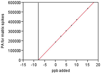
Figure 1 - For the matrix spikes, plot of response versus the added concentration.
Black vertical line shows the determination of blank’s level (8.06 ppb) via
standard addition. PA = peak area.
The above work showed that the three conditions for proceeding
with Step 3 were met. For the standard-addition procedure, the
responses (peak areas) obtained for each matrix spike (including
the “blank”) were plotted versus the spike concentration. A
straight line with OLS fitting was appropriate; thus, it was reasonable
to proceed with the standard-addition calculation. Extrapolation
of the line showed that ppb ≈ –8.1 when PA = 0 (see Figure 1).
In this illustration, the results from the various steps supported each
other and it was reasonable to assume that the “blank” contained
~8 ppb of fluoride, plus-or-minus ~1 to 2 ppb. Not bad agreement
with the known value of 10 ppb!