As was discussed in the previous column of this series (in the January 2003 issue of American Laboratory), calibration is a procedure that imperfectly transforms a response into a useful measurement. It follows that there is uncertainty associated with any straight-line calibration (or, for that matter, with any calibration “curve,” such as a fitted exponential function). Hence, if one conducts repeated calibration experiments, different coefficients for each experiment’s equation will be the result. (One hopes that the differences are relatively small.) An example is shown in Figure 1.
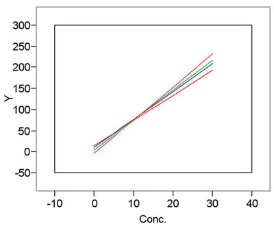
Figure 1 - Example of calibration curves resulting from
multiple calibration experiments using the same method,
equipment, and concentrations of standards.
In order to quantify the uncertainty in any given calibration line, the concept of uncertainty intervals is needed. In statistics, there are three types of uncertainty intervals:
- Confidence intervals give the uncertainty in an estimate of a population parameter. (Note: A parameter is the true, but unknown, value of a key descriptive numerical quantity, either for a function or for the distribution of a population. Examples are the true mean and standard deviation of daily rainfall in Kalamazoo, or of pork-belly futures.) Confidence intervals are not appropriate for reporting measurements, which are not parameters.
- Prediction intervals give the uncertainty in one future measurement. These intervals are the most widely utilized for reporting measurements and will be used throughout this series of articles.
- Statistical-tolerance intervals quantify the uncertainty in a chosen percentage of k future measurements (k may be infinite). Such intervals are appropriate for reporting measurements, but are more complex to interpret. Also, to create statistical-tolerance intervals, tables of critical values are needed but are difficult to find.
(Note: The width of the interval increases as one progresses from (1) to (2) to (3), since there is more accounting for variation with each step.)
For a given calibration curve, the prediction interval consists of a pair of prediction limits (an upper and a lower limit) that bracket the curve. Each limit has a user-chosen level of significance associated with it (e.g., 2.5% or 0.5%). The confidence level for the prediction interval is 100% minus the sum of these two levels. Although these two levels are typically the same, they do not have to be. For a straight line (SL), the prediction interval (for the measurement, in concentration units) used at a given value of y is:
 ,
,
where x = (y–a)/b; a = the intercept of the line on the y-axis; b = the slope of the line; t = Student’s t; dof = degrees of freedom (for a SL, dof = [n – 2]); γ = the significance level associated with the limit in question (i.e., either the upper or the lower limit); RMSE = the root mean square error (often used to estimate the measurement standard deviation, which is the statistic actually needed here); n = the number of data points in the calibration design; xavg = the mean of the x values in the calibration; and Sxx = the corrected sum of squares = Σ[(x – xavg)2]. Prediction intervals capture the uncertainty in the: 1) calibration-line slope, 2) calibration-line intercept, and 3) response.
The above equation was not given with the intent that the reader should memorize it. However, calibration experiments can be designed more intelligently if the equation is understood. Generally, one has some control over some of the terms in the equation. Knowing how the terms’ sizes will affect the value of the interval can be a guide to wise planning. The next paragraphs will discuss the equation in some detail.
In general, the formula says that the line’s uncertainty is a function of three main components:
- RMSE, which is an estimate of the measurement standard deviation; i.e., the inherent variation in the measurement system, typically the component that is the most responsible for uncertainty.
- A square-root term that can be no smaller than 1.
- Student’s t, which is the “penalty factor” that must be included since the true variation in the system is unknown. For 99% confidence, Student’s t approaches 2.33 as n increases. (Most people are familiar with the ±3 sigma approximation. The name comes from the fact that this method calls for 7 or 8 replicates [i.e., 6 or 7 degrees of freedom after the standard deviation is calculated]; with dof = 6 or 7, t is approx. 3 at 99% confidence. Similarly, ±2 sigma approximates 95% confidence.)
Table 1 - Student’s t table*
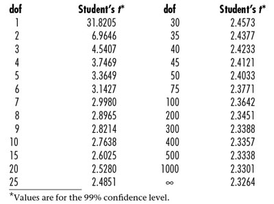
For a given instrumental method, the choice of calibration design will not have a significant effect on RMSE. The only ways to decrease RMSE significantly are: 1) to obtain a method or instrument with less variation, or 2) to report an average of m independent measurements, reducing RMSE by a factor of the square root of m. However, the other two main components are affected by the choice of design. Student’s t is affected by the number of degrees of freedom (i.e., the number of data points). As n increases, t decreases. However, a quick look at a Student’s t table shows that there are diminishing returns even for moderate values of n (Table 1). As can be seen, the biggest gain is in moving from a dof of 1 to a dof of 5~10. Once n degrees of freedom exceed 20 or so, there is little reduction in t.
It should be noted that there is a huge penalty if calibration is done using only one measurement on each of three concentrations of standards (Table 1). In this situation, dof is only 1; thus t is 31.8. If each standard were simply run in triplicate, the dof would rise to 7 and t would drop to 3. The decision to run more than the “bare minimum” design will greatly affect the prediction interval.
The third component of the formula is the square-root expression. The number of data points, n, affects this part also. Since n is in the denominator, (1/n) can be reduced by driving n higher, an action already favored because of the effect on t. Finally, [(x – xavg)2/Sxx)] depends on two things. The closer x = (y – a)/b is to xavg, the narrower the interval (see the numerator); in addition, the wider the calibration range, the narrower the interval (see the denominator). Actually, Sxx is maximized when the calibration design consists of half the points at the low value, and half at the high value, with none in between. However, this design is not recommended because it is does not allow for model validation (e.g., determining if curvature is present, meaning that the straight-line model should be challenged). (Calibration design and model validation will be discussed in more detail beginning in the next article.)
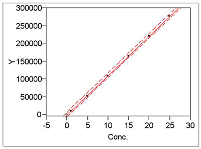
Figure 2 - Example of a calibration line enveloped by its
upper and lower prediction limits (i.e., upper and lower
curves, respectively).
In summary, one can decrease the size of the prediction interval by: 1) keeping n high, and 2) making the range of the calibration design as large as possible (provided that the model is plausible for the entire range). Once the calibration experiment is conducted, the prediction interval can be plotted along with the calibration line. An example is shown in Figure 2. While all three lines appear more or less parallel in this plot, the interval lines may flare out at either end. This phenomenon occurs most often when only a small number of data points are available.
It should also be pointed out that, technically, the interval applies to the y-values (i.e., the responses). In calibration, one wants to know the uncertainty in any concentration predicted from the line (i.e., the x-values). The simplest technique, which applies to all types of models, is to plot the curve and interval via statistics software. Then, the width of the interval can be measured graphically against either axis.
Mr. Coleman is an Applied Statistician, Alcoa Technical Center, MST-C, 100 Technical Dr., Alcoa Center, PA 15069, U.S.A.; e-mail: [email protected]. Ms. Vanatta is an Analytical Chemist, Air Liquide-Balazs™ Analytical Services, Box 650311, MS 301, Dallas, TX 75265, U.S.A.; tel: 972-995-7541; fax: 972-995-3204; e-mail: [email protected].