In the last installment in this series, it was suggested that a rule-of-thumb for calibration designs was five-by-five, (i.e., five replicates of each of five concentrations), for a total of 25 data points. If the user were restricted to only 25 analyses, variations in the five-by-five might be desirable to meet various analytical goals. Table 1 illustrated five possible 25-point designs that might be utilized for various calibration experiments. It was recommended that the reader try to analyze the designs to decide when each might be useful. The present paper discusses the reasoning behind each possibility. Please note that the range of measurements shown in the design examples (Table 1) is for simplified illustration purposes only. A range of 0–8 can represent 0–80, 0–800, etc.
Table 1 - Sample calibration designs
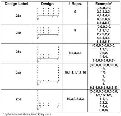
Design 25a in Table 1 contains five replicates at each of five concentrations that are equally spaced. This arrangement is a “vanilla” approach. It allows for modeling of the standard deviation (there are sufficient replicates at each of a sufficient number of concentrations to determine how the standard deviation is behaving). Since the levels are equally spaced, this design would be applicable if the following conditions hold: 1) curvature is not expected in any part of the range, 2) there is no need for an extremely low detection limit, and 3) the desired calibration range is limited (i.e., excluding zero, the range does not span more than one or two orders of magnitude).
In Table 1, 25b, one of the higher concentrations has been sacrificed in order to have an additional low-end standard. Again, there are five replicates at each level and modeling of the standard deviation is possible. However, an additional low-level concentration allows for easier detection of curvature near zero. As will be described in a future column, this design would also promote a lower detection limit.
The user of 25c would be interested in very precise predictions at the two extremes of the range, or a heightened ability to detect a difference in measurement variation between these two extremes. These goals are suggested because of the high number of replicates at the ends. The design does generate some data for detecting low-end curvature, although only triplicates are available for the three “interior” concentrations. A low detection limit is also promoted here, and standard-deviation modeling is possible.
The design in 25d is similar to 25c in that both have many replicates at each end of the concentration range. However, in this fourth case, higher priority is placed on detecting (but not modeling) a difference in measurement variation between the extremes of the range, since interior replicates have been sacrificed to gather even more data at the two extreme concentrations. Lack of interior replicates makes curvature detection difficult.
The final design, 25e, has the same number and spacing of levels as 25d. However, in this last example, some replicates at the high end have been conceded in order to have triplicates for all interior concentrations. This alteration would be needed if the user wanted data for standard-deviation modeling. There is still a need for high precision at the low end (hence the large number of replicates at the lowest concentration). This design also generates data for detecting curvature at the low end, since five levels are tightly grouped in that area and replicates are available. In addition, a low detection limit is promoted.
Again, it should be emphasized that the above examples are just that—possibilities for constructing a calibration protocol. If there is a limit on the total number of analyses that can be included in the experiment (as was assumed in the above), then trade-offs may be necessary in order that some of the goals be achieved. If a variety of objectives are important, the trade-off may have to be an increase in the number of analyses in the design.
To illustrate some designs that have been used in actual research projects, three protocols will be presented from the authors’ work. These examples cover a variety of situations, ranging from analyses that challenged the sensitivity of the instrument to cases that demanded the dilution of the sample prior to testing. In all instances, a minimum of five replicates was made at each concentration. Each replicate was made on a different day and not all days were back-to-back. For each replicate, the standards were prepared fresh and analyzed in random order. This arrangement was chosen in order to incorporate day-to-day variability into the design. It should be kept in mind that no “magic formula” was used to set up any of these calibration experiments. Each protocol was the result of careful consideration of the goals of the project and a thoughtful discussion of how these aims might be accomplished.
The first example involved the low-level determination of several contaminants in deionized water. The primary range of concern was around 50 ppt (parts per trillion), a level that pushed the sensitivity of the instrument, even with concentration techniques. However, reliable data also were desired out to about 150 ppt. For each analyte, nothing was known a priori about the standard deviation or curvature. Since the low concentrations formed a critical area, several concentrations in that range were included (a strategy that also allowed for detection of low-end curvature). The final design contained a blank (mandatory for trace-level work) and eight non-zero concentrations: 25, 37.5, 50, 62.5, 75, 100, 150, and 200 ppt; the last concentration was included so that 150-ppt samples could be analyzed without extrapolation. Eight replicates of this set of standards were analyzed. To summarize, this protocol allowed for: 1) determination of very low concentrations, 2) detection of low-end curvature, 3) standard-deviation modeling, and 4) analysis of samples out to 150 ppt.
The next calibration design was for an assay method. The procedure was used to ensure that each of two components was between 5 and 10 wt% in the formulation. Instrument sensitivity was not a problem (the sample actually had to be diluted before analysis was possible); thus detection limits were not an issue. Clearly, the main goal was to have high precision at the specification limits (at 5 and 10 wt%). The design had to overlap these two values for two reasons. First, doing so would bracket these critical numbers, and second, such a curve would permit reliable reporting of slightly out-of-specification results, thereby providing data for reworking any out-of-spec solutions. The final design consisted of 11 concentrations, each of which was prepared and analyzed (in random order) on each of eight different days. The exact levels were 3.5, 4.5, 5.0, 5.5, 6.5, 7.5, 8.5, 9.5, 10.0, 10.5, and 11.5 wt%; i.e., a modified equi-spaced design. The modification was to insert the two specification limits (i.e., 5.0 and 10.0 wt%). This number of levels and replicates enabled the detection of curvature as well as standard-deviation modeling.
The third design was developed for a project in which the analytes of interest could range from 1 to 98% (wt/wt). As in the above example, preanalysis sample dilution was necessary. All that was required was a calibration curve that could provide reasonable estimates of sample concentrations. Curvature at the low end was suspected. The levels chosen were 1, 2, 4, 8, 25, 50, 75, and 98%. This design allowed for modeling of standard deviation (five replicates of each of eight standards were included). In addition, there were closely spaced levels in the low end, where curvature was a distinct possibility.
The next installment in this series will summarize what has been presented thus far and permit the authors to clarify and correct some of the earlier material. The paper will also set the stage for a discussion of the next main topic: calibration diagnostics.
Mr. Coleman is an Applied Statistician, Alcoa Technical Center, MST-C, 100 Technical Dr., Alcoa Center, PA 15069, U.S.A.; e-mail: [email protected]. Ms. Vanatta is an Analytical Chemist, Air Liquide-Balazs™ Analytical Services, Box 650311, MS 301, Dallas, TX 75265, U.S.A.; tel: 972-995-7541; fax: 972-995-3204; e-mail: [email protected].