This month's article will conclude the three-part series explaining calibration diagnostics. There are seven basic steps to this procedure:
- Plot response versus true concentration
- Determine the behavior of the standard deviation of the response
- Fit the proposed model and evaluate R2adj
- Examine the residuals for nonrandomness
- Evaluate the p-value for the slope (and any higher-order terms)
- Perform a lack-of-fit test
- Plot and evaluate the prediction interval.
In the previous two installments (American Laboratory, Nov 2003 and Feb 2004), steps 1–2 and steps 3–4, respectively, were detailed. The final three steps are discussed below.
Step 5: Evaluate the p-value for the slope (and any higher-order terms)
When a model is fitted to a data set, values are determined for the various coefficients (the intercept and the slope, for a straight line). An additional coefficient (with associated p-value) is calculated for each higher-order term that is added to the model.
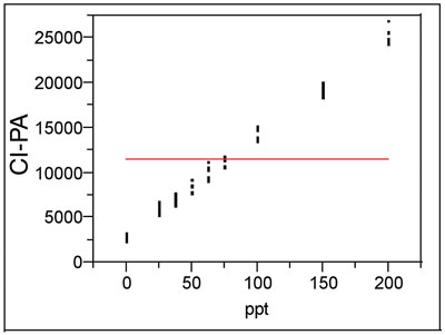
Figure 1 - Plot of a straight line with zero slope through the mean of a data set. This model is the
null hypothesis for testing the adequacy of a straight line.
When a software package calculates the p-value for the slope, it must start with a null hypothesis. In this case, the starting assumption is that a straight line with zero slope through the mean of the responses is adequate to explain the data (see Figure 1). In most calibration work, the higher the concentration, the greater the response from the instrument. Consequently, the slope will (nearly) always be positive. Thus, the null hypothesis constitutes an inadequate model in comparison to a regressed straight line (even if such a line is not a completely adequate model for the data). As a result, the p-value for the slope will inevitably be <0.01. In other words, assuming the null hypothesis is true, the odds of obtaining the given set of calibration data (purely by chance) would be extremely low. Consequently, the starting assumption is rejected and the proposed model (the alternative hypothesis) is accepted instead.
A similar evaluation is made of the p-values associated with any higher-order terms. In such cases, the null hypothesis is the model that is one order lower (e.g., the straight line is the starting hypothesis for testing a quadratic model). For example, if a second-order model is to be considered as a possibility, then the p-value for the quadratic term should be <0.01; if not, then overfitting has occurred and a straight line is adequate. For the data set in Figure 1, a straight line (ordinary least squares [OLS] is needed as the fitting technique) has a significant p-value (<0.0001). The residual plot, which is not shown, reveals a random pattern, consistent with an adequate straight-line model. Further confirmation of the straight-line selection comes when a quadratic term is added; the p-value for x2 is seen to be quite high (0.8406), indicating that the term is not significant and therefore not needed.
Step 6: Perform a lack-of-fit (LOF) test
It is possible to conduct a formal LOF test, which generates a p-value that is useful in calibration diagnostics. The null hypothesis for this test is that there is no lack of fit. In other words, if the model under consideration is adequate, then there is no lack of fit and a high p-value should result. (Recall that a high p-value means that the starting assumption is not rejected.) Typically, a p-value of greater than 0.05 is taken to mean that there is no lack of fit and that the proposed model is adequate. For example, with the data set in Figure 1, a straight line with OLS fitting has a LOF p-value of 0.9050, giving additional confirmation of the adequacy of that model.
This test works in conjunction with the residual pattern, which above was shown to be a good indicator of the adequacy of a given model. The residual plot is a more informal and somewhat subjective diagnostic. The LOF test is a formal statistical procedure that does not require the practice or interpretation needed for residual analysis. Another helpful attribute is that the LOF test does not require the user to specify a particular alternative model, such as a quadratic or exponential relationship. Both the LOF test and residual analysis require replicate data for at least some of the concentrations in the data set. When used together, the two diagnostics give the user a high degree of confidence in his or her ability to choose an adequate model.
Step 7: Plot and evaluate the prediction interval
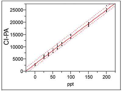
Figure 2 - Plot of a calibration curve (straight-line model via OLS fitting) with its associated prediction
interval (at 95% confidence).
The first goal of any calibration experiment is to find an adequate model for the data. The resulting calibration curve is used to predict analyte concentration in unknown samples. The second goal (which is of equal importance) should be to calculate the corresponding prediction interval. (See installment 4, American Laboratory, Mar 2003, for a discussion of prediction intervals.) For a given confidence level, this interval tells the user the overall uncertainty associated with a given prediction from the curve. The analyst and the customer should calculate and evaluate this uncertainty, since only by performing such an analysis can they decide if the calibrated method is adequately precise. An example of a calibration curve and its prediction interval (at 95% confidence) is shown in Figure 2.
Mr. Coleman is an Applied Statistician, Alcoa Technical Center, MST-C, 100 Technical Dr., Alcoa Center, PA 15069, U.S.A.; e-mail: [email protected]. Ms. Vanatta is an Analytical Chemist, Air Liquide-Balazs™ Analytical Services, Box 650311, MS 301, Dallas, TX 75265, U.S.A.; tel: 972-995-7541; fax: 972-995-3204; e-mail: [email protected].