This article is the first in a series of real-world calibration analyses. Since the research of one of the authors (L. Vanatta) is dedicated almost exclusively to ion chromatography, the examples in this column are from that field. However, the procedures are not specific to chromatography, or even chemistry; they are generally applicable and mirror the diagnostic steps outlined in articles 8, 9, and 10 (American Laboratory Nov 2003, Feb 2004, and Mar 2004, respectively).
The analyte (chloride) is one of the species included in a trace-level procedure for anions in deionized water. The calibration design was presented in installment 6 (American Laboratory July 2003). Eight replicates of a blank and each of nine standards— 25, 37.5, 50, 62.5, 75, 100, 150, and 200 ppt—have been analyzed. Straight-line (SL) calibration using ordinary-least-squares (OLS) fitting has been proposed for the data.
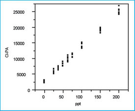
Figure 1 - Scatterplot of all 72 chloride responses plotted versus
their respective true concentrations.
Step 1: Plot response versus true concentration
After all 72 data points have been collected, the responses are plotted versus the true concentrations. The scatterplot in Figure 1 exhibits a pattern typical of the suggested SL/OLS combination, and no suspect data points are seen. However, any suspect data or a nonlinear (i.e., nonstraight-line) relationship will become more apparent in Step 4 below (i.e., during the examination of the residual plot).
Step 2: Determine the behavior of the standard deviation of the response
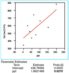
Figure 2 - For the chloride responses at each concentration, the straight-line/OLS plot of the standard deviation versus the true concentration. The
p-value of the slope (shown in bold and labeled “ppt” in the “Term” column)
is above the significance threshold of 0.01. Thus, the slope is not considered
significant and OLS is the appropriate fitting technique.
First, the standard deviation of the responses is calculated for each concentration. These results are plotted versus true concentration and modeled with a straight line using OLS. The resulting plot (plus the parameter estimates for the line) is given in Figure 2. The only information needed in this step is the p-value for the slope of the line; if the value is above 0.01 (i.e., 1%), then the slope is not considered statistically significant. In other words, the noisiness of the response (in absolute terms) does not change significantly as a function of concentration. Such constancy, which is the desired outcome, indicates that OLS is the appropriate fitting technique. (Note: Weighted least squares should be used if the data indicate that the response's standard deviation is increasing with concentration, thereby violating one of the key assumptions behind OLS.)
In Figure 2, the slope's p-value (denoted by the Term "ppt") of 0.0270 is shown in bold. Because this value is above the "threshold," OLS is appropriate for the fitting technique.
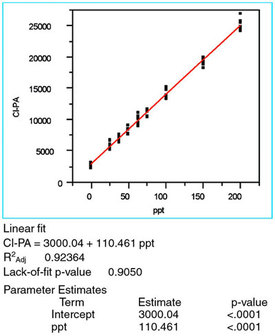
Figure 3 - The straight-line/OLS plot of the chloride responses versus
the true concentration. Also included are 1) the equation for the line, 2)
R2adj, 3) the lack-of-fit p-value, and 4) the parameter estimates (i.e., the
intercept and slope, the latter of which is designated "ppt"), and their
associated p-values.
Step 3: Fit the proposed model and evaluate R2adj
Once the fitting technique has been tested, the model can be examined. Figure 3 shows the original scatterplot modeled with a straight line via OLS. The R2adj of 0.92 is less that the traditionally desired 0.99+; however, as discussed in Part 9 (American Laboratory Feb 2004), R2adj is a relatively weak calibration-diagnostics tool. Thus, this R2adj is sufficiently high to avoid signaling an alarm.
Step 4: Examine the residuals for nonrandomness
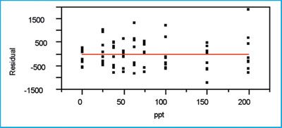
Figure 4 - The residual plot associated with the SL/OLS curve in
this example.
The residual pattern (see Figure 4) appears to be random about the zero line. If the model were inadequate, a distinct shape (e.g., parabola) would be noted. The variation in the responses does appear to be increasing somewhat with concentration, but the standard-deviation modeling performed above indicates that the increase is not statistically significant.
Step 5: Evaluate the p-value for the slope
The slope's p-value is less than the cutoff of 0.01 (see Figure 3), meaning that the starting assumption (i.e., a straight line parallel to the x-axis explains the data adequately) should be rejected. This low p-value is a good result and it is expected for any calibration data; it demonstrates that the analytical method has an adequate signal-to-noise ratio.
Step 6: Perform a lack-of-fit test
The lack-of-fit test (which assumes no lack of fit as the starting hypothesis) has a p-value (0.9050; see Figure 3), which is greater than the cutoff of 0.05. Thus, there is no indication that a term is missing from the model.
Step 7: Plot and evaluate the prediction interval
Figure 5 shows the data's scatterplot with not only the SL/OLS curve but also the prediction interval (confidence level = 95%). As is typical for data in which the response's standard deviation is constant (i.e., OLS is appropriate) and n is greater than approximately six, both lines of the prediction interval are nearly straight and nearly parallel to the calibration curve. This interval gives the uncertainty associated with the next sample's concentration predicted from the curve.
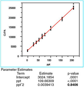
Figure 6 - Plot of a quadratic/OLS plot of the chloride responses versus
the true concentration. The significant result is the p-value (0.8406,
shown in bold) for the quadratic term (i.e., the “ppt^2” entry in the
“Term” column of “Parameter Estimates”). Since this value is above the
cutoff of 0.01, the term is not significant, meaning that a second-order
polynomial overfits the data and should not be used.
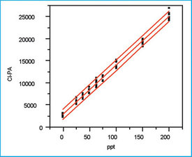
Figure 5 - SL/OLS plot of response versus concentration,
along with the prediction interval when the confidence level is 95% (α =
β = 2.5%).
In this example, if the graph is enlarged in any given concentration region, the uncertainty is measured graphically to be ± ca. 10 ppt. It isup to the user to decide if this amount of variation (and confidence level) is acceptable for the method at hand; statistics cannot make this decision!
For completeness, a quadratic model is applied to the data using OLS (see Figure 6). While the R2adj and the lack-of-fit p-value are both acceptable, the p-value (0.8406, shown in bold) for the quadratic term is insignificant, meaning that the term is not needed. Thus, the straight-line/OLS combination is appropriate for these data (a conclusion supported by the associated p-value for the lack-of-fit test).
Mr. Coleman is an Applied Statistician, Alcoa Technical Center, MST-C, 100 Technical Dr., Alcoa Center, PA 15069, U.S.A.; e-mail: [email protected]. Ms. Vanatta is an Analytical Chemist, Air Liquide-Balazs™ Analytical Services, Box 650311, MS 301, Dallas, TX 75265, U.S.A.; tel: 972-995-7541; fax: 972-995-3204; e-mail: [email protected].