This month’s installment is the third in a series of real-world examples of calibration diagnostics. The analyte is phosphate and is one of the components of an ion-chromatographic assay method. Details of the calibration design can be found in Part 6 (American Laboratory July 2003). Eight replicate injections were made of each of nine standards (i.e., 3.5, 4.5, 5.0, 5.5, 6.5, 7.5, 8.5, 9.5, 10.0, 10.5, and 11.5 wt%). A straight-line model with ordinary-least-squares (OLS) fitting was proposed to fit the data.
Step 1: Plot response vs true concentration
The scatterplot for the response data is seen in Figure 1. All points appear to be well-behaved, and there is no evidence of curvature. As always, though, these observations will be tested via the following diagnostics.
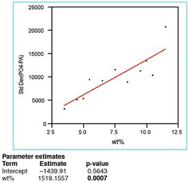
Figure 2 - Response standard deviation has been plotted versus true
concentration and modeled with a straight line, using OLS as the fitting
technique. The low p-value (0.0007, in boldface) for the slope indicates
that the standard deviation does increase with concentration.
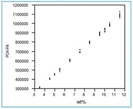
Figure 1 - Scatterplot for the phosphate data. No outlying points are
seen and the postulated straight-line model seems plausible. PO4-PA
stands for phosphate’s peak area.
Step 2: Determine the behavior of the standard deviation of the response
In Figure 2, the standard deviation of the responses is plotted versus true concentration; a straight line has been fitted using OLS. The desired statistic is the p-value for the slope of the straight line (i.e., the boldfaced value under “p-value” for the term “wt%”). For these data, this statistic is 0.0007 (i.e., 0.07%), well under the cutoff of 1%; thus, the starting hypothesis of constant standard deviation is rejected and the alternative hypothesis (i.e., that the standard deviation increases with increasing concentration) is accepted. The practical result of this rejection decision is that OLS should not be used as the fitting technique for peak-area-vs-concentration calibration; weighted least squares (WLS) is chosen instead.
With WLS, the response data are weighted so that the noisy data are not allowed to influence the regression process as much as are the precise data. For each observation, the formula for the weight is the reciprocal square of the standard deviation at that concentration, divided by the mean of all the reciprocal squares. The standard deviation is calculated using the formula obtained in the standard deviation plot (i.e., –1439.9 + [1519.16 × wt%]).
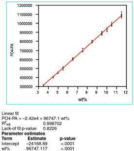
Figure 3 - Scatterplot (same as in Figure 1) fitted with a straight-line
model, using WLS as the fitting technique. The statistics of R2adj, lack-of-fit
p-value, and p-value for the slope (i.e., “wt%” under “Parameter estimates”)
all indicate that this model is appropriate for these data.
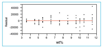
Figure 4 - Residual pattern that relates to Figure 3.
Step 3: Fit the proposed model and evaluate R2adj
The proposed model of a straight line is fitted to the data (using the WLS results from Step 2 above) and adjusted R2 is examined. As seen in Figure 3, this value is acceptably high; R2adj= 0.9987 = ~99.9%.
Step 4: Examine the residuals for nonrandomness
For some concentrations, the zero line for the residual plot is either above or below the mean of the residuals (see Figure 4). In any case, the offsets are not severe in this data set. However, the spread of the points does appear to be increasing with concentration. This “trumpet-effect” observation is consistent with the decision in Step 2 to use WLS as the fitting technique. There are no other striking anomalies (e.g., bunching, outliers, curvature, or trends).
Step 5: Evaluate the p-value for the slope
As expected, the p-value for the slope is well under 1% (see the “wt%” term under “Parameter estimates” in Figure 3). In other words, a straight-line regression model is better than a straight line parallel to the x-axis.
Step 6: Perform a lack-of-fit test
Since the starting assumption for this test is that there is no lack of fit, a high p-value (i.e., greater than 0.05) means that the chosen model is adequate. The value of 0.8226 (see Figure 3) indicates that a straight line is adequate, a conclusion supported by the residual pattern in Figure 4, discussed in Step 4.
Step 7: Plot and evaluate the prediction interval
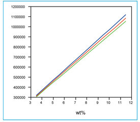
Figure 5 - Straight-line/WLS curve (from Figure 3) along with its
prediction interval (at 95% confidence). Note the flaring of the prediction
interval. This effect occurs because WLS “compensates” for
the increasing standard deviation of the responses.
All of the above results support the use of a straight line with WLS fitting to model the phosphate data. The resulting calibration curve and its associated prediction interval (at 95% confidence) are given in Figure 5. Unlike the previous two examples (where OLS was the fitting technique), the prediction interval here does flare as concentration increases. This phenomenon is the primary result of having a nonconstant response standard deviation and is to be expected. If there is more uncertainty (i.e., a higher standard deviation) at higher concentrations, then the prediction interval should be wider. As always, only the user can decide if the width of the prediction interval is acceptable for the situation at hand.
As a last step, the data in Figure 1 were fitted with a quadratic model, using WLS (plot not shown). The p-value for the quadratic term was found to be 0.5594, well above the cutoff of 0.01. Thus, this higher-order model is not needed and, if used, would result in overfitting of the phosphate data.
Mr. Coleman is an Applied Statistician, Alcoa Technical Center, MST-C, 100 Technical Dr., Alcoa Center, PA 15069, U.S.A.; e-mail: [email protected]. Ms. Vanatta is an Analytical Chemist, Air Liquide-Balazs™ Analytical Services, Box 650311, MS 301, Dallas, TX 75265, U.S.A.; tel: 972-995-7541; fax: 972-995-3204; e-mail: [email protected].