This fourth real-world example of calibration diagnostics comes from the same study as did Part 13 (American Laboratory, Sept 2004). The analyte this time is fluoride, another component of an ion-chromatographic assay method. Details of the calibration design can be found in Part 6 (American Laboratory, Jul 2003). Eight replicate injections were made of each of 11 standards (i.e., 3.5, 4.5, 5.0, 5.5, 6.5, 7.5, 8.5, 9.5, 10.0, 10.5, and 11.5 wt%). Since previous experience has taught that fluoride peak-area (F-PA) data often exhibit quadratic behavior, this second-order model was proposed to fit the data, using ordinary least squares (OLS) as the fitting technique. Had quadratic behavior not been expected, a straight-line model and OLS fitting would have been assumed. The calibration diagnostics then would have been applied to that fit.
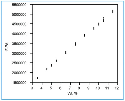
Figure 1 - Scatterplot for the fluoride data. Data are well-behaved. Standard deviation appears to increase with concentration.
Step 1: Plot response vs true concentration
The scatterplot (response data vs true concentration) is shown in Figure 1. All points appear to be well-behaved. However, the response data appear to become noisier as concentration increases (e.g., notice the middle and next-to-highest concentrations relative to the lowest two). The curvature issue is difficult to resolve and may be obscured by the changing noise. The following calibration diagnostics will determine the appropriateness of these observations.
Step 2: Determine the behavior of the standard deviation of the responses
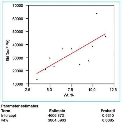
Figure 2 - Plot of response standard deviation vs true concentration. Data have been fitted with a straight line, using OLS fitting. The p-value (0.0085, boldfaced) of the slope is less than 0.01, meaning that the standard deviation is increasing with concentration.
The standard deviation of the responses is plotted versus true concentration (see Figure 2). As is customary, a straight line has been fitted using OLS. The statistic of interest is the p-value for the slope of the straight line (i.e., the boldfaced value under “Prob > |t|” for the term “wt%”). In this example, this statistic is 0.0085 (i.e., 0.85%). As was the case for phosphate in the previous example, this value is below the recommended cutoff of 1%. When the p-value is this low, the standard deviation is declared nonconstant, meaning that OLS should not be used as the fitting technique; instead, weighted least squares (WLS) is chosen.
As was seen in the previous example, a weight is calculated for and applied to the response data at each concentration. The formula for the weight is the reciprocal square of the estimated standard deviation at that concentration, divided by the mean of all such reciprocal squares. An appropriate way to estimate the standard deviation is to use the equation from the regression results for this step. As seen in Figure 2, the formula is [4606.872 + (3804.5903 * wt%)].
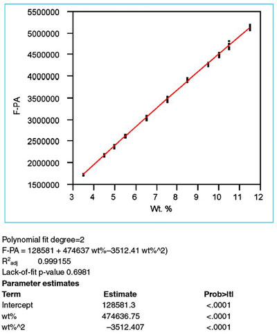
Figure 3 - Scatterplot (as seen in Figure 1) fitted with a quadratic model, using WLS as the fitting technique. The statistics of R2adj, lack-of-fit p-value, and p-values for the x- and x-squared terms (i.e., “wt%” and “wt%^2,” respectively, under “Parameter estimates”) all indicate that this model is appropriate for these data.
Step 3: Fit the proposed model and evaluate R2adj
The proposed model of a second-order polynomial is fitted to the data (using the WLS results from step 2 above). Adjusted R2 is found in Figure 3 and is 0.9992 (i.e., ~99.9%). Although this statistic is quite high, it should be emphasized again that this yardstick is the weakest tool in the calibration-diagnostics procedure. By itself, R2adj should not be taken as assurance that the chosen model is the most appropriate possible model.
Step 4: Examine the residuals for nonrandomness
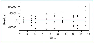
Figure 4 - The residual pattern for the quadratic model fitted in Figure 3.
Figure 4 shows that, in general, the zero line passes through each concentration’s residuals at approximately their mean values. This characteristic indicates that the chosen model (i.e., a quadratic) is appropriate. The choice of fitting technique, though, is a different matter. The spread of the residuals becomes larger as concentration increases, indicating that the standard deviation of the responses is not constant. This observation agrees with the decision above (in step 2) to use WLS instead of OLS as the fitting technique.
Step 5: Evaluate the p-value for the slope
For a quadratic model, there are two terms of interest (i.e., the x-term itself and the x-squared term). The p-value for each of these terms (and especially the quadratic) should be less than 0.01. Otherwise, the model overfits the data. In this case, both statistics meet the criterion (see “wt%” and “wt%^2” under “Parameter estimates” in Figure 3).
Step 6: Perform a lack-of-fit test
This test assumes that there is no lack of fit with the chosen model. Thus, a high p-value (i.e., greater than 0.05) is required. Otherwise, a term (or terms) is assumed to be missing. The value of 0.6981 in Figure 3 shows that a second-order polynomial is adequate. This finding reinforces the conclusions drawn from the residual pattern (in step 4).
Step 7: Plot and evaluate the prediction interval
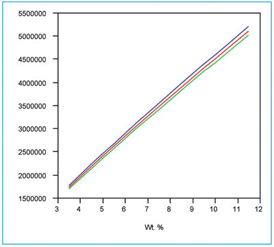
Figure 5 - The quadratic/WLS curve (as seen in Figure 3) along with its prediction interval (at 95% confidence). The interval flares because the response standard deviations increase with concentration.
The above results are consistent with each other and lead to the choice of a quadratic model with WLS fitting for these fluoride data. The calibration curve and its associated prediction interval (at 95% confidence) are shown in Figure 5. As was seen with phosphate in the previous example, the prediction interval flares with increasing concentration. In both cases, this shape is the expected result when the response’s standard deviations change with concentration. As is always the case, only the user can decide if the width of the prediction interval is acceptable for the application under consideration.
As a last step, the data in Figure 1 were fitted with a cubic model, using WLS (the plot is not shown). The p-value for the cubic term was found to be 0.2254. Since this value is higher than the cutoff of 0.01, the additional term is not needed. In other words, the use of a cubic model would overfit these fluoride data.
Mr. Coleman is an Applied Statistician, Alcoa Technical Center, MST-C, 100 Technical Dr., Alcoa Center, PA 15069, U.S.A.; e-mail: [email protected]. Ms. Vanatta is an Analytical Chemist, Air Liquide-Balazs™ Analytical Services, Box 650311, MS 301, Dallas, TX 75265, U.S.A.; tel: 972-995-7541; fax: 972-995-3204; e-mail: [email protected].