Measurement is at the heart of what analytical chemists do on a routine basis. People want to know how much X is in a particular sample, S, or at what proportion X can be found in S (i.e., a number, expressed in appropriate units). Usually, several steps (e.g., sample preparation, instrument calibration, chemical processing, and “data reduction”) are involved in arriving at the “how much” answer. Each of these steps can affect both the level and the variability of the reported value. Thus, measurement should be envisioned as a multistep process whose ouput is numbers.
Measurements always vary. When a sample is measured twice or when two identical samples are measured, it is rarely the case that the two measurements are the same. Therefore, an honest and complete report of a measurement involves an estimate of uncertainty. Sometimes, we can refine steps of the measurement process to reduce this uncertainty, perhaps to a tolerably low level. However, we can never eliminate variability totally; it is inevitable.
The simplest nontrivial way to express this situation with an equation is as follows:
yi= f(xi)+ εi + bias
where yi is the measurement i (e.g., peak area); f(xi) is the function relating xi to yi; xi is the true value (e.g., concentration); and εi is the “noise” or random error. Bias is the systematic error, which may not be constant over the range of x values. As an estimate, bias is equal to [true predicted] and loosely may be called “inaccuracy.”
Measurements will fall along the real-number line, which (on the low end of the working range) can be divided into segments, as illustrated in Figure 1.
In segment (a), M is indistinguishable from a concentration of 0. In other words, M is a “nondetect.” In (b), M is a detection, but confidence in the ability to detect is low. Once M is as high as segment (c), M is a detection, and detection is likely. However, the measurement value is very noisy. Finally, when M is as high as segment (d), M can be reported as a numerical measurement value that has a high level of confidence.
At this point, we would like to introduce a topic that is often ignored, yet should be fundamentally important to all users and producers of numerical measurements. This subject is uncertainty intervals. As stated earlier, all measurements will vary. As chemists, we need to be able to assess the amount of this variation before we can decide if the reported value is “tight” enough for our purposes, or those of our customers/colleagues. However, we typically ignore this aspect, rationalizing that we cannot be bothered by such qualifiers: “Just give us the result, please.”
This (unqualified) approach opens the door to making decisions that are unwise—and potentially costly. As a simple example, assume that the criterion for releasing a shipment of a chemical depends on the shipment’s having a contaminant level of less than 10 ppm. If the laboratory report shows the measured value as 9 ppm, we probably will accept the material. If we had known that the variation in the measuring process was ±0.1 ppm, would we have made the same decision? Probably, assuming our requirements were not too stringent. What if the variation had been ±5 ppm? In this case, we most likely would not have been so quick to use the chemical. We also probably would question the analytical method used to do the analysis.
The point is that we constantly need to be asking, “How reliable is a given measurement?” and “How should I estimate the reliability?” Statistics can give us the tools needed to calculate reliability in the form of an appropriate uncertainty interval. (This topic will be discussed in detail in later articles.) Thus, we must think about our situation and decide how much variation we can tolerate in our measurements. If we are dealing with processes that have life-or-death consequences (e.g., purity of a drug or integrity of an airplane engine), then our tolerance of uncertainty will be quite low. On the other hand, if we just need a ballpark evaluation of the concentration of a given sample ingredient, then we might not care about the noisiness of our measurement system.
While we need to be concerned that our results are “tight” enough for our purposes, we should also avoid requesting more precision than is necessary. Otherwise, we will be paying (probably both in time and money) for a measurement system that is much more expensive than is necessary. The answer to the generic question of “How ‘good’ a number do you need?” should involve a conscious tradeoff of costs and risks, not simply be “How ‘good’ a number can you give me?”
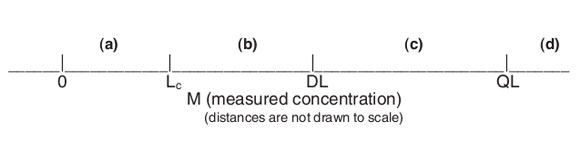
Figure 1 - Real number line, where Lc is the critical level and concentration that serves as a statistical “critical level,” i.e., any measurement below Lc cannot be (statistically) distinguished from zero, because of measurement noise; DL is the detection limit and concentration below which a response cannot be detected reliably; and QL is the quantitation limit and concentration below which a numerical measurement value cannot be reported reliably.
It cannot be emphasized enough that statistics can only give one the tools and statistical analyses that allow one to evaluate one’s data. Only the user can decide if the results have acceptable variability. Remember, people make decisions, based on thoughtful consideration of statistically sound data analyses.
Another way to look at these ideas is to return to the thoughts presented at the end of our introductory column (American Laboratory, September 2002). The two questions that are at the heart of calibration, detection, and quantitation, were discussed. The first query asks, “What is the appropriate estimate of the measurement uncertainty?” The second asks, “What risk level is acceptable?” In the first case, statistics provides the answer. However, only you and your colleagues and customers can decide the second issue. Remember these two questions, since they are critical to every analytical method and will often be at the center of this series of articles.
Mr. Coleman is an Applied Statistician, Alcoa Technical Center, MST-C, 100 Technical Drive, Alcoa Center, PA, U.S.A.; e-mail: david.coleman@ alcoa.com. Ms. Vanatta is an Analytical Chemist, Air Liquide-BalazsTM Analytical Services, Box 650331, MS 301, Dallas, TX 75265, U.S.A.; tel.: 972-995-7541; fax: 972-995-3204; e-mail: [email protected].