As was stated at the end of Part 50, this current installment will be the last in the “Statistics in Analytical Chemistry” series. The mission of this article is to correct mistakes and clarify confusing or incomplete statements from past manuscripts. My thanks to alert readers who have brought some of these instances to my attention! Every attempt has been made to catch all technical mistakes. However, if anyone finds additional problems, please let me know!
Part 4—In the paragraph beginning, “For a given calibration curve…”: The prediction interval being discussed is for a straight line (SL) using ordinary least squares (OLS) as the fitting technique. The formula (x – xavg)2 should be changed to: [(yi – yavg)/b]2. Furthermore, the corrected expression is an approximation; the exact formula is in the y-direction and is given by:
Part 5—Under “Study design”: Change “After steps 11–3” to “After steps 1–3.”
In the next-to-the-last sentence of that last paragraph, it is better to say, “the standard deviation is not trending with concentration,” since there are occasions when this statistic decreases as concentration increases.
Part 8—In Step 2: If the SL/OLS fit of the data reveals a positive slope, the standard-deviation data should be refitted using weighted least squares (WLS). The formula for the new line should be used to calculate the final weight (assuming that one iteration has not changed the coefficients too much).
Part 9—In the paragraph beginning, “When the proposed model…”: The reference to installment 2 is incorrect; the usefulness of residual patterns was not discussed until Part 9.
Part 11—In the paragraph beginning, “The analyte (chloride)…”: There are nine total standards (a blank and eight non-zero standards).
In all figures, “Cl-PA” refers to the peak area for chloride.
Part 13—In the paragraph beginning, “This month’s installment…”: There are eleven total standards.
Part 14—In Step 5: As long as the p-value for the higher(est) model term is less than 0.01, the term is significant (i.e., the p-values for lower-order terms are not critical).
Part 16—In the paragraph beginning, “Figure 2 displays…”: Delete the clause, “and is approximately symmetric in concentration.”
Part 18—In the caption for Figure 3: The lack-of-fit p-value is 0.0072.
In the paragraph beginning, “The appropriate calibration line…”: Change the end of the second sentence to “the prediction-interval width is approximately the same (in the y-direction) throughout the calibration range.”
Part 19—In the paragraph beginning, “To evaluate recoveries…”: There are ten concentrations (i.e., a blank and nine non-zero standards).
Part 22—In the paragraph beginning, “Because of popular demand…”: Delete the parenthetical expression, “(i.e., comparing the amount of residual variation at each concentration with the amount of variation in residual means between concentrations).”
Part 24—In the definition of “LOF”: Delete the clause, “compares the amount of residual variation at each concentration with the amount of residual variation between concentrations.”
The following definitions should be added to the Glossary:
Alpha (α)—The probability of obtaining a false positive (PFP) when measuring a blank.
Beta (β)—The probability of obtaining a false negative (PFN) when measuring a low-level standard.
Part 25—In item 5 under Step 3: The significance (or lack thereof) of the higher(est)-order term’s p-value is the only statistic that is of concern. (See Part 14 above.)
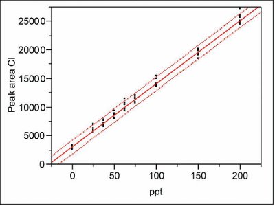
Figure 3 corrected
Part 30—The plot shown in Figure 3 is a duplication of Figure 4 and thus is incorrect. The correct Figure 3 is shown here (see “Figure 3 corrected”).
Part 31—Equation (1) applies to a straight-line model with OLS as the fitting technique.
Equation (19) must be used iteratively, since RxD contains xD.
Part 33—In the paragraph beginning, “In the last installment…”: 0.748 should be 0.742.
Part 37—In the paragraph beginning, “The standard deviation is the most basic…”: “x” should be “xi,” where i goes from 1 to n (i.e., the change is in the formula for SD).
In the paragraph beginning, “In any regression analysis, …”: The negative exponent should be deleted from the formula for SEslope.
In the paragraph beginning, “As an illustration of the above…”: “(more places than needed for these stats)” should be deleted.
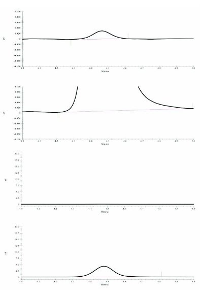
Part 42 figures corrected
Part 42—The chromatograph tracings are not dark enough to read easily. Darker versions for Figures 1, 2, 3, and 4, respectively, are shown here (see “Part 42 figures corrected”).
Parts 42 and 43—When comparing replicate analyses of standard to a true blank, seeing if the uncertainty interval contains zero is statistically proper. However, when comparing any two data sets where neither set is zero, a t-test should be conducted to determine if there is a statistically significant difference between the means.
Part 46—In the paragraph beginning, “For SSError, the starting point…”: p = the total number of parameters; delete “(p).” (As usual, n represents the total number of data points.)
Part 47—In the paragraph beginning, “The first unwise practice…”: The admonition always to regress y on x should be qualified. The noisier data should be regressed on the well-behaved data. In most cases, the concentrations (typically labeled “x”) are well-behaved when compared with the responses (typically labeled “y”). However, there are instances where the concentrations contain more variability than do the responses; in such cases, the concentrations should be regressed on the responses.
In the caption for Figure 1, “interval” should be changed to “limit.”
The author would like to thank David Coleman for helpful conversations about t-tests.
To my readers:
It has been an amazing ten-plus years!!
As this column comes to a close, I owe a debt of gratitude to many people. First and foremost, I thank you, dear readers, for your interest in the subject matter and support of the publication of the articles!! Without all of you, the series would have ceased long ago. Those of you who have contacted us have kept us sharp and helped shape the direction of the column; thank you for your input!
Several specific people and organizations also are on my thank-you list. Above all, I am very grateful to David Coleman for all the statistical training he has given me since 1995. Without his patience and willingness to teach, I never could have taken on this project. Most of all, I thank him and his family for their friendship!
Pittcon® also deserves applause for making short courses a part of the conference (since it was through that program that David and I met) and for continuing to let David and me teach our class. The annual sessions help us keep up on chemists’ statistical challenges in the lab.
In addition, without the blessing of Bob Stevenson and the late Brian Howard of American Laboratory, this column never would have gotten off the ground. Their encouragement and friendship have been invaluable. In addition, I thank everyone at American Laboratory/Labcompare for all the hard work and patience they have devoted to effecting publication of each article. I have met or talked with many of these people, and all of them have become good friends.
Lastly, although I wrote the articles on my own time, I am indebted to three former managers for their enthusiastic support of my research projects and of my ideas for investigating sound statistics. These men are: 1) Tom Talasek of Texas Instruments and 2) Tony Schleisman and Joe Hoffman of Air Liquide.
In closing, I want to wish each reader the richest of blessings, plus a long and rewarding life. Your allowing me into your world has greatly enriched my life, and I am very thankful to all of you! Until we meet again, Happy Number-Crunching!!
Lynn Vanatta is an Analytical Chemist; e-mail: [email protected].