Consider the following algebraic equation:
Since this single expression has three unknowns, there are many possible solutions; a single exact solution cannot be found. In other words, there is not a unique set of x, y, and z values that will satisfy the equation. However, values can be assigned to the variables, up to a point. If, for example, x is set to 10 and y is set to 20, then the result is one equation in one unknown. At this stage, z cannot be chosen at will. Once x and y have been assigned, then z is “locked in” by the constraints of the equation. The only alternatives are: 1) to allow x or y to “float” so that z can be given a value, or 2) assign z and then replace the equal sign with a not-equal sign. There is no way around the following restriction: only (n-1) of the n unknowns in a single equation can be replaced with numbers. The equation will determine the value of the last (nth) variable.
While the above may seem trivial, this algebraic fact is often ignored (at least subconsciously) when it comes to detection limits. As was discussed in the previous article (Part 26, American Laboratory 2007, 39[12], 24–25), the world of detection can be described by one equation in three unknowns, which are: 1) the detection limit (DL), 2) the probability of false positives (PFP, known as α), and 2) the probability of false negatives (PFN, known as β). Once any two of the three have been chosen, the third is automatically set by the equation.
For a given set of low-level data (with which a detection limit is logically associated), this equation allows the user to investigate the trade-offs among the three variables. A graphical representation is possible; such a plot is known as a Receiver Operating Characteristic (ROC) curve (or set of curves). The U.S. military developed these plots. Aluminum sheets that will be used in aerospace applications must be tested to determine the presence of flaws. ROC curves allow the user to model the probabilities of detection or nondetection.
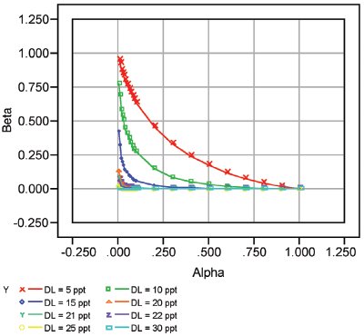
Figure 1 - Chloride ROC curves. On any ROC curve, the desired location is the lower left-hand corner (i.e., α and β both have been chosen to be low). For this analyte, that goal can be reached only if the detection limit is no lower than about 20 ppt.
An ROC curve traditionally has α (i.e., PFP) on the x-axis and (1-β) (i.e., 1-PFN*) on the y-axis. However, most people work mainly with α and β themselves, so in this series of articles, β will be plotted versus α for ROC curves. Once these two axes have been established, a family of curves can be generated. Each curve is associated with a particular value for the DL. An example plot is given in Figure 1. Eight chloride DLs have been plotted. These limits range from a low of 5 parts per trillion (ppt, w/w) to a high of 30 ppt. In any detection-limit situation, the goal is to “live” in the lower left-hand corner of the graph. Only in this region are α and β both controlled at low levels (typically, less than 5% each). However, not all DLs will allow such control. In this example, the curve can enter this corner only if the DL is at least ca. 20 ppt.
It is possible, though, that a lower DL (e.g., 5 ppt) needs to be maintained. In such a situation, the user can see the trade-offs between the false-positive probability (or rate) and the false-negative rate. As can be seen from the plot, if α is kept very low, then β is very close to 1 (the user can ignore this latter reality, but it is there nevertheless). This result is simply due to the constraints of the algebraic equation that related the DL, α, and β for this set of data. If the DL is chosen to be 5 ppt, then α and β cannot both be set to whatever values are desired.
Figure 1 actually is related to the data that were presented in Calibration Example 1 (Part 11, American Laboratory2004, 36[10], 40–45), where the matrix was deionized water. (In Part 11, the regression [or calibration] diagnostics revealed that a straight line [SL] with ordinary-least-squares [OLS] fitting was appropriate to explain the data.)
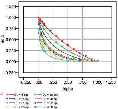
Figure 2 - Nitrite ROC curves for low DLs. This plot for nitrite uses the same detection-limit values as were used in Figure 1. However, even though nitrite exhibits a chromatographic response similar to that of chloride, the nitrite data are noisier. Thus, none of the values is high enough to drive the related curve into the lower left-hand corner.
Nitrite data from the same study were presented in Calibration Example 2 (Part 12, American Laboratory2004, 36[14], 38–40). (Again, an SL with OLS fitting was adequate.) An ROC plot (showing the curves for the same set of DLs as were used in Figure 1) is given in Figure 2. Note that even at the maximum value shown (i.e., 30 ppt), α and β cannot be simultaneously held to less than 5%. In other words, the lower left-hand corner cannot be reached.
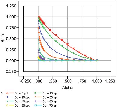
Figure 3 - Nitrite ROC curves for higher DLs. Only by allowing the detection limit to rise to at least 40 or 50 ppt can the ROC curve be driven into the lower left-hand corner.
Only by allowing the DL to rise to higher values can the ROC curve pass through this desired location (see Figure 3). In other words, a DL of at least ca. 50 ppt must be allowed for nitrite. Just because analytes (here, chloride and nitrite) are part of the same calibration study (and generate data that can be explained adequately by the same combination of model and fitting technique) does not mean that the detection-limit situation will be the same for both. Ultimately, the width of the prediction interval is key to the way the ROC curves will behave for a given analyte.
Even if the user is willing to sacrifice either a low α or a low β in the quest for lower and lower DLs, there is a practical limit to this process. The risk that one is willing to take of being wrong can be quantified by the sum of α and β. Thus, the overall confidence level one “enjoys” is [100% – (α + β)]. As the DL is pushed lower and lower, the ROC curve moves farther and farther away from the lower left-hand corner, and (α + β) becomes larger and larger. Eventually, this sum will reach 100%. At that extreme, the confidence level sinks to zero. In other words, the ROC curve is a straight line from (α = 100%) to (β = 100%) (i.e., the chance line). With such a situation, one might as well be picking an extremely low DL at random!
If it is desirable to have a DL pass through the lower left-hand corner of the ROC plot, then how does one ensure such an outcome? The answer to this question will be addressed in the next several installments.
*The expression (1-PFN) is the probability of true positives (PTPs), since given the presence of the analyte, the only two possible outcomes are that the substance is not detected or that it is detected. The PTP is known as the power to detect (a true positive).
Mr. Coleman is an Applied Statistician, Alcoa Technical Center, MST-C, 100 Technical Dr., Alcoa Center, PA 15069, U.S.A.; e-mail: [email protected]. Ms. Vanatta is an Analytical Chemist, Air Liquide-Balazs™ Analytical Services, Box 650311, MS 301, Dallas, TX 75265, U.S.A.; tel.: 972-995-7541; fax: 972-995-3204; e-mail: [email protected].