In the previous article (Part 22, American Laboratory, June/July 2006), the details behind the lack-of-fit (LOF) test were discussed. However, the principles behind degrees-of-freedom (dof) calculations were deferred until this current installment. To begin, a brief review of LOF purpose and details will be given, including a slightly different approach to the calculation.
The LOF test is intended to determine whether there is statistically significant evidence that a model is inadequate. Recall that the LOF test is based on errors. The total error associated with a regression data set is a combination of the pure error (i.e., error associated with the data, independent of any model) and the lack-of-fit error (i.e., error associated with the inadequacy of a model to explain the data). The LOF test compares the former to the latter. Thus,
Pure Error + LOF Error = Total Error
It should be noted that each type of error may also be referred to in the literature as “error sum of squares” (SS) or “error corrected sum of squares” (CSS).
Calculation of these error terms involves the squaring of a difference (or residual) associated with each data point, and then summing all of these squares. Consider the contribution of a single data point (i.e., the instrumental response obtained by analyzing a given concentration of standard) to each of these errors. The pure error is the square of the following difference: response itself minus the mean response for all of that concentration’s responses. The LOF error is the square of the difference: mean response for that concentration minus the predicted response from the chosen model. The total error is the square of the difference: response itself minus the predicted response from the chosen model.
As the equation implies, once any two of the three errors have been calculated, the third can be determined. Traditionally, statisticians (and statistical software packages) have conducted an F-test (to which type the LOF test belongs) by calculating LOF error indirectly (i.e., from the difference between the total and the pure errors). It was from this perspective that Part 22 was written.
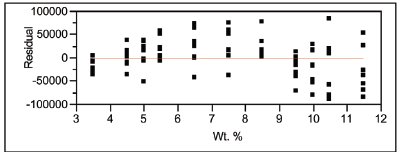
Figure 1 - Residual pattern associated with the results in Table 1.
For purposes of understanding degrees of freedom in the LOF test, it is helpful to consider each error’s calculation independently. To illustrate the process, the straight-line/weighted-least-squares (SL/WLS) fit of the previous example (see Part 22) is used again. In that data set, 8 replicates of each of 11 concentrations were analyzed, giving a total of 88 data points. Table 1 and Figure 1 show the LOF statistics and the residual pattern, respectively.
In determining the number of available dof, the first step is to determine how many data points are in the data set under consideration; each data point will contribute one dof. The next step is to decide how many statistics are being estimated from these data points; one dof is “expended” for each such calculation. The dof available is the difference between these two numbers. Often, it is step one that causes consternation. For each dof tally, the user must start at the beginning and decide what data set is actually involved.
Consider first the dof for the pure error. This error depends only on the distance of each data point from the mean at that concentration. Each distance (i.e., difference) is squared and then all of the squares are summed. Thus, all of the data points (which are independent of each other) are needed for the calculation. Hence, each point contributes to the initial pool for dof. In this example, the total is 88. However, a mean must be calculated for each concentration. In this case, there are 11 concentrations, so 11 dof are expended, giving a net of 77 dof for pure error.
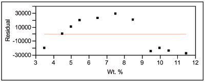
Figure 2 - Residual pattern associated with the results in Table 2.
In determining the dof for the LOF error, it is useful to realize that there is more than one way to determine any model’s equation. One approach is to fit the model to the actual data set, as has been done in all of the examples in this series of articles. Another path is to replace each response with the mean of all the responses at that particular concentration (which results in the same parameter estimates for the regression, but bogus confidence intervals and p-values). Since LOF error is calculated from the distance of the mean to the model’s line, the residuals for this “means-only” path represent the needed distances. Table 2 and Figure 2 show the LOF and residual results for the SL/WLS fit when the means are used at each concentration. Since the response (i.e., the mean) is the same at each x-value, there is no pure error, so all of the error is due to lack-of-fit.
When each of the 88 data points is replaced with its associated mean, each mean counts only once in the dof realm. This restriction is due to the fact that no new piece of information is added to the pool when a mean is replicated. Thus, no additional contribution is made to the initial dof tally. Thus, only 11 data points (i.e., the 11 means) are available. However, two dof are expended when the straight line is fitted to the data (i.e., an intercept and a slope are calculated). Thus, the net dof for LOF is 9.
For the total error, the squares of all the residuals from the model’s fit are summed. Thus, all of the data points are needed and each contributes to the initial dof pool; as with the pure error, 88 is the starting number. Once again, though, the SL model must be fit in order to generate residuals. Thus, a slope and an intercept are calculated from the data, meaning that two dof are expended; the net dof for total error is 86.
One detail has been overlooked in the above. The issue is the effect of calculating a weight on the dof for each error. As can be seen from the LOF tables, statistical- software packages assume there is no effect of weighting. However, recall from Part 8 of this series (American Laboratory, November 2003) that weight calculations involve fitting a straight-line model to the standard-deviation data; this process uses two additional degrees of freedom. These two dof should be “charged” to some account. The bad news is that statisticians have not resolved this matter among themselves, and a discussion of the debate is beyond the scope of this column. The good news, though, is that the effect of these dof “charge-outs” on the LOF-test results is insignificant, assuming a well-designed calibration (or any regression) study has been used.
Mr. Coleman is an Applied Statistician, Alcoa Technical Center, MST-C, 100 Technical Dr., Alcoa Center, PA 15069, U.S.A.; e-mail: [email protected]. Ms. Vanatta is an Analytical Chemist, Air Liquide-Balazs™ Analytical Services, Box 650311, MS 301, Dallas, TX 75265, U.S.A.; tel.: 972-995-7541; fax: 972-995- 3204; e-mail: [email protected].