Because of popular demand from readers, this installment will discuss the principles and calculations that underlie the lack-of-fit (LOF) test. Recall from part 10 (American Laboratory, March 2004) that this test helps the user decide if the selected model explains the data adequately. The test is based on the residual “pattern,” which was discussed in part 9 (American Laboratory, February 2004), and is a formal, numerical evaluation of one aspect of the pattern (i.e., comparing the amount of residual variation at each concentration with the amount of variation in residual means between concentrations).
To understand lack of fit, it is helpful to consider first the objectives of calibration (or of regression performed on any set of y-versus-x data). In the ideal situation, each true concentration (or x value) would lead to replicate responses that are exactly the same and the adequate model would exactly intersect all of these replicate data points. In such a case (which never happens!), there is no bias (i.e., systematic variability) and no random variability. The response for each true concentration is completely predictable, and the model fits “perfectly.”
In the real world, of course, there is always random scatter of the data; thus, essentially never will two responses for each true concentration be exactly the same. This random error is called “pure error,” since it is inherent in the data themselves and will exist no matter what model is fitted (or if no model is applied). The typical technique for quantifying pure error is to calculate the associated sum of squares, which is equivalent (except for scaling by 1/[n–1]) to calculating a variance. The procedure is to calculate 1) the mean response at each concentration; 2) the difference between each mean and each of the associated raw responses; and, finally, 3) the sum of the squares of each difference. In other words:
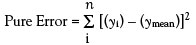
where yi = the ith response, ymean = the mean response at yi’s concentration, and n = the total number of data points. (It should be noted that when the mean is subtracted before squaring, as it is here, the result sometimes is referred to as the “corrected” sum of squares.)
In the above “real-world” situation, the desirable circumstance again is that an adequate model will pass exactly through the mean of each concentration’s set of responses, since such an occurrence would mean that there is no systematic bias. Even this phenomenon virtually never occurs. Thus, the question is, “Do the residual means deviate from zero enough to suggest there is bias?” If the answer is “yes,” then the model is inadequate. In an inadequate-model situation, there are two contributions to the overall error: 1) the pure error that is due to the random, inherent scatter in the data; and 2) deviations of the means at each true concentration (i.e., the inability of the model to explain totally the mean behavior). This combined error is called “total error” and can be quantified by calculating the associated sum of squares. The process is 1) calculate the residual (i.e., observed response minus predicted response) for each data point, and 2) sum the squares of all the residuals. In other words:
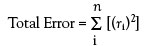
where ri = the residual for the ith response.
Of necessity, the total error will be larger than the pure error. The difference is the error that is due to the (possible) inadequacy of the model and is called “lack of fit.” In other words:
Lack of Fit = (Total Error) – (Pure Error)
The question, then, is how the size of the LOF error compares with the size of the pure error. If the lack of fit is “sufficiently” small compared to the inherent noise of the data, then the model can be considered to be adequate (LOF is never zero). On the other hand, if the LOF portion “dominates” the pure error, then the model is not an appropriate one for the data. To compare these two errors, an F-test is used; this test compares the ratio of two variances. However, before the ratio is calculated, the variances must be scaled by the degrees of freedom available to each value. The ratio of these scaled variances is then taken to an F-table to get a p-value, which is the value that is used in the LOF portion of calibration diagnostics.
While the above discussion explains the basic concept of lack of fit, it omits one important issue (i.e., the matter of weights). Recall from part 8 (American Laboratory, November 2003) that a fitting technique must be chosen. If the standard deviation of the responses does not trend with concentration, then ordinary least squares (OLS) is appropriate; otherwise, weighted least squares (WLS) is needed. In WLS, the well-behaved data are weighted such that they have greater influence on the regression than do the noisier data. The weights that are calculated for fitting the model also must be taken into account in the LOF test. Thus, for WLS,
where wi = the weight for the ith raw response.
To illustrate the above concepts, consider the data that were discussed in Calibration Example 4 (American Laboratory, December 2004). In this data set, the standard deviation did trend with concentration, so weights were calculated and used in fitting the model. A straight-line (SL) fit was tried first. The lack-of-fit table is shown in Table 1. Each entry in the “Sum of squares” column was calculated using the formulas (including weights) given above. The “DF” column shows the number of degrees of freedom associated with each type of error. While a derivation of these DF results is in order, a full explanation is rather lengthy and will be saved for the next article in this series. For now, the reported numbers will be accepted “on faith.”
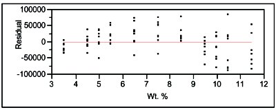
Figure 1 - Residual pattern associated with the straight-line model, using weighted-least-squares fitting.
The “Mean square” column contains the results of dividing each “Sum of squares” entry by the appropriate “DF,” and the “F ratio” is the LOF mean square divided by the pure-error mean square. When this ratio (4.1174) is taken to an F-table, the p-value (“Prob>F” in the table) is 0.0002. Recall that the LOF test assumes there is no lack of fit associated with the model. Thus, a low p-value (with this test, a value of less than 0.05) indicates that there is lack of fit. In other words, the LOF error is significantly larger than the random or pure error. As expected, the residual pattern (see Figure 1) supports this conclusion, since the LOF test is based on the residuals.
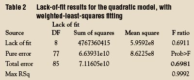
Note that while the above LOF results indicate that the SL model is inadequate, this test gives no guidance in choosing an alternative model; the residuals must be examined to make that decision. The pattern in Figure 1 is parabolic in nature, a shape that suggests a quadratic model be tried next. The LOF data for this polynomial (again with WLS fitting) are shown in Table 2. This time, the p-value is 0.6981, which is well above the cutoff of 0.05. With this model, the LOF error (or the bias) has been reduced to the point that its contribution to the total error is small and the pure error dominates. Thus, a second-order polynomial is considered to be adequate to explain the data. The residual pattern shown in Figure 2 is in agreement with this decision.
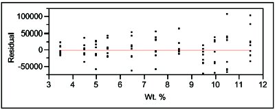
Figure 2 - Residual pattern associated with the quadratic model, using weighted-least-squares fitting.
Mr. Coleman is an Applied Statistician, Alcoa Technical Center, MSTC, 100 Technical Dr., Alcoa Center, PA 15069, U.S.A.; e-mail: [email protected]. Ms. Vanatta is an Analytical Chemist, Air Liquide-Balazs™ Analytical Services, Box 650311, MS 301, Dallas, TX 75265, U.S.A.; tel.: 972-995-7541; fax: 972-995-3204; e-mail: [email protected].