The previous two installments have discussed the issue of nonideal recovery, a problem that occurs in many analytical methods. Since internal standards (ISs) are commonly used, a statistical protocol was presented for evaluating IS candidates. Subsequently, a recovery-curve alternative was outlined, as this approach overcomes many of the drawbacks to internal standards. However, several questions remained unanswered at the end of this second discussion. This article will answer those queries, comment on the related subject of blanks, and remark on the technique of standard addition.
In the previous discussion (American Laboratory, February 2006), an example involving six analytes was used. An appropriate model and fitting technique were determined for each set of recovery data, and the equations for the various lines were given. In no case was the y-intercept exactly zero or was the slope exactly one.
This situation should come as no surprise with real data, but since recovery curves are postcalibration and after blank subtraction, it is reasonable to have “slope = 1” and “intercept = 0” as starting hypotheses (i.e., the perfect recovery curve, which will be tested statistically). The questions that were raised previously were 1) Does the confidence interval (at a given confidence level) include one and zero, respectively, and 2) does it matter if either answer is “no”?
The first task is to determine the width of the uncertainty interval around both the slope and the intercept. For these calculations, the standard error (SE) of the desired parameter estimate is needed. (The standard error is the estimate of the standard deviation associated with a particular parameter estimate.) However, the width of the interval is not simply the parameter estimate plus or minus the SE. The confidence level associated with this interval is not fixed, but is chosen by the user. Since the SE is also an estimate and not the true value (which can never be known), the SE must be multiplied by the appropriate value of Student’s t. In this discussion, a confidence level of 95% has been chosen. Because the interval is divided into a “plus” and a “minus” portion, the 0.05 uncertainty must be divided in half as well. There are 72 data points in each analyte’s data set. Initially, there is one degree of freedom (dof) for each data point. However, one dof is lost for each parameter estimate that is calculated. Thus, a net of 70 degrees of freedom remains for a straight line and 69 for a quadratic model. At the 0.025 uncertainty level with approximately 70 dof, Student’s t is approximately 1.99. Multiplying the standard errors by this value, followed by subtracting from and adding to the parameter estimates, gives the intervals listed in Table 1. Terms whose intervals do not include one (for the slope) or zero (for the intercept) are marked with double asterisks. (The quadratic term for chloride is not discussed here.)
Table 1 Parameter-estimate results for the six analytes*
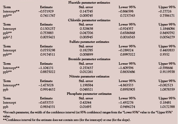
What could lead to a slope that is significantly different (statistically) from one? The short answer is that analyte is lost (and sometimes gained) during the course of the analytical method. For most methods, there are numerous opportunities for this loss or gain to happen (e.g., digestions, dilutions or concentrations, transfers). Thus, a nonunity slope is not uncommon and is why chemists generate recovery curves in the first place.
What could lead to an intercept that is significantly different (statistically) from zero? The answer often lies in part with the blank. As was mentioned in the previous article, recovery curves are constructed after any blank values have been subtracted. (In general, it is best to average the blank responses before performing the subtraction. However, in some cases, subtracting the day’s blank from that day’s spike-recovery data might be more appropriate. Such was thought to be the case in this example, which involved the digestion of 30% hydrogen peroxide and the determination of trace anions. The laboratory atmosphere was thought to be a possible contributor to any positive blanks. Since the air’s composition probably varied from one day to the next, individual values were thought to be closer to the true.) Once the appropriate blank value has been subtracted from each nonzero standard, the blank values have served their purpose and are not included in the concentration range of curve. Thus, in the H2O2 example, each resulting recovery curve actually was between 10 ppb (the lowest standard) and 40 ppb (the highest concentration). Therefore, the regression line had to be extrapolated in order to calculate an intercept (and its associated confidence interval). In other words, the line between 10 ppb and zero was based on no data.
A similar situation occurs when there is no blank response that can be integrated. Three of the analytes (fluoride, bromide, and phosphate) fell into this category. In these situations, no peak-area values were obtained for the matrix blank. Thus no net (predicted) ppb values were entered into the data table. (It is not advisable to force the fit through zero, since all data have noise!) The regression results for no entries are the same as if rows for the blank had not even been entered into the table.
In reality, the concept of a y-intercept is an artificial construct. The statistical result from performing regression is that a constant term results. While it is tempting and fairly logical to tie this value with the chemical concept of a blank’s response, doing so can lead to misleading concerns about “nonzero” numbers. The best thing to remember is the basic rule that regression curves should not be extrapolated!
Although this series of articles deals primarily with the statistical aspects of chemical analysis, a brief discussion of blank selection is in order. In low-level analyses, blanks are critical to obtaining meaningful data. Thus, care must be taken in defining what the appropriate blank will be for a given study. The goal of recovery (or calibration) studies is to capture all of the variability that can reasonably be expected to occur in day-to-day operations. If any part of the procedure might contribute (either positively or negatively) to the value of the response from a sample or standard, then the blank should be taken through those steps as well. Thus, the pure solvent that is used for diluting samples may not be a sufficient blank in a calibration study. In a recovery study, an analyte free (if possible) matrix should be used as the basis for the blank.
One other subject (i.e., standard addition) merits a brief discussion. This technique involves analyzing an unknown sample as is, plus spiked separately at one or more concentrations. Responses are plotted versus spike concentration. A straight line is regressed through the data points and then extrapolated back to the negative x-axis (i.e., to y = 0). This intersection represents the estimate (ignoring the negative sign) of the analyte’s concentration in the original sample. In many ways, standard addition is very similar to the recovery curves when there is a positive response for the blanks. In both instances, there are no response data between the blank’s analyte amount (which is unknown) and zero. However, standard addition is not an advisable protocol. First, there typically is the tendency to prepare and analyze only a few spike concentrations, and to do so without replicates. Second, and more importantly, to make extrapolation feasible, only a straight-line model is realistic, even if the data exhibit curvature. In the end, though, matrices that cannot be obtained in “uncontaminated” form present a situation for which there is no good measurement procedure.
Mr. Coleman is an Applied Statistician, Alcoa Technical Center, MST-C, 100 Technical Dr., Alcoa Center, PA 15069, U.S.A.; email: [email protected]. Ms. Vanatta is an Analytical Chemist, Air Liquide- Balazs™ Analytical Services, Box 650311, MS 301, Dallas, TX 75265, U.S.A.; tel.: 972-995-7541; fax: 972-995-3204; e-mail: [email protected].