In Part 19 of this series (American Laboratory Dec 2005), the use of an internal standard (IS) was discussed and an example was given. This article presents an alternative that overcomes many of the drawbacks and limitations common to an IS. The topic is recovery curves. The laboratory work involved in generating these plots is very similar to the IS-evaluation steps presented earlier. Also, the instrumental response (to a given combination of analyte concentration and matrix composition) is again assumed to be relatively stable.
The protocol is as follows. First, design and conduct a calibration study (using pure solvent) over the applicable concentration range. For the data from each analyte, select an appropriate model and fitting technique, using the calibration diagnostics outlined in previous articles in this series; evaluate the prediction intervals (at the desired confidence level) to be sure they are tight enough.
Second, design and perform a spiking study (including a blank and covering the same concentration range as above), in which the spikes are made into the matrix under consideration. Determine the recovered concentrations, using the pure-solvent calibration curve for the respective analytes; perform blank subtraction, if appropriate.
Third, plot the recovered concentrations versus the true (spike) concentration. These graphs are the basis for the recovery curves. As a first approximation, a straight-line (SL) model with ordinary-least-squares (OLS) fitting can be used for each analyte’s data. For each line’s equation, the y-intercept represents the “bias part” of recovery, while the slope represents the proportional recovery that is achieved. The prediction interval gives the overall statistical uncertainty for the entire method (including both calibration- and matrix-related effects), at the desired confidence level. Either the plot or the equation can be used to convert the recovered concentrations back to the true concentrations. These latter values can then be reported along with the uncertainty given by the prediction interval.
To be more complete in the third step, an SL/OLS combination should not be assumed. Instead, calibration diagnostics should be used to choose an adequate model and fitting technique for each analyte’s data. This more rigorous approach will be used in the example that follows.
In order to illustrate the concept of recovery curves, the determination of anions in digested hydrogen peroxide is used again (see American Laboratory Dec 2005 for details of the calibration design). Recoveries for fluoride, chloride, sulfate, bromide, nitrate, and phosphate are examined; in each case, the concentration range is 10–50 ppb. Blank subtraction was performed for analytes when necessary. The calibration-diagnostic results are found in Table 1; the plots in Figures 1–6 show the actual recovery curves, along with their prediction intervals (at 95% confidence).
Table 1 - Calibration-diagnostics results for the six recovery curves
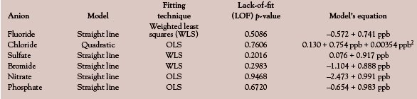
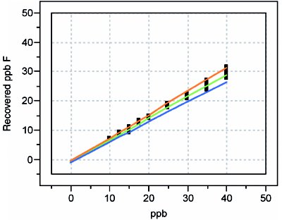
Figure 1 - Recovery curve for fluoride.
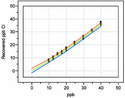
Figure 2 - Recovery curve for chloride.
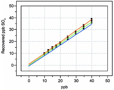
Figure 3 - Recovery curve for sulfate.
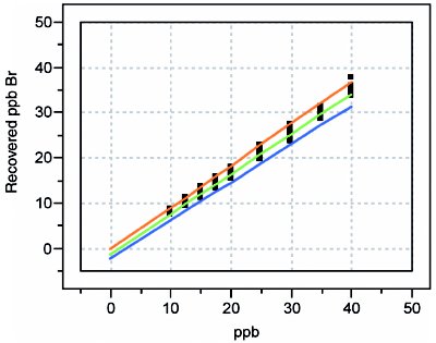
Figure 4 - Recovery curve for bromide.
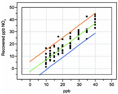
Figure 5 - Recovery curve for nitrate.
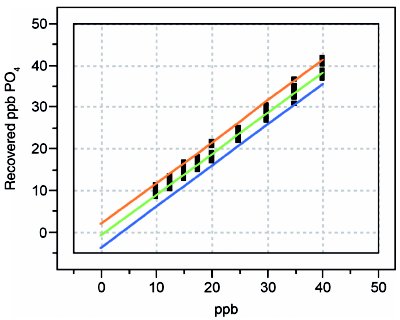
Figure 6 - Recovery curve for phosphate.
Two observations are noteworthy. First, the model and fitting technique are not the same for all analytes, even though all six anions were part of the same recovery study. As with calibration curves, the data should be allowed to “speak for themselves.” It would be risky to assume that an SL/OLS combination is appropriate for everything (although this assumption is commonly made).
Second, simply having an analyte that may display a high percent recovery (e.g., nitrate, with a slope of 0.991) does not mean that the uncertainty in the measurement is acceptable. Note that the half-width of nitrate’s prediction interval is ca. 10 ppb. On the other hand, fluoride exhibits the opposite situation (i.e., a low recovery, but a tight prediction interval). Fluoride’s ca. 75% recovery would be unacceptable to many chemists. However, from a statistical perspective, this behavior is much preferred to that of nitrate because of the difference in the prediction-interval widths. In all cases, reporting true-ppb values along with the uncertainty is preferred. It is misleading merely to accept the recovered value as long as it is within a specified range (typically, between 85 and 115% recovery), since the user has no idea 1) where in that range the true value lies, and 2) how noisy the data are.
These data sets also raise several questions. First, for each analyte, does the uncertainty interval (at a given confidence level) for the y-intercept include 0? In other words, is the estimated bias statistically indistinguishable from 0? Second, similarly, does the uncertainty interval (again, at a given confidence level) for the slope include 1? In other words, apart from bias, is the recovery statistically indistinguishable from the ideal of 100%? Third, how much does it matter if the answer to either of the above questions is “no”? The answers to these questions will be addressed in the next installment.
Mr. Coleman is an Applied Statistician, Alcoa Technical Center, MSTC, 100 Technical Dr., Alcoa Center, PA 15069, U.S.A.; e-mail: [email protected]. Ms. Vanatta is an Analytical Chemist, Air Liquide-Balazs™ Analytical Services, Box 650311, MS 301, Dallas, TX 75265, U.S.A.; tel.: 972-995-7541; fax: 972-995-3204; e-mail: [email protected].