The previous several articles have dealt with calibration-study design and calibration-diagnostic procedures. These discussions have centered on two specific quantities: 1) the true concentrations of the calibration standards, and 2) the instrumental responses to these various standards. In the six examples that were detailed, the responses were the raw peak areas generated by an ion chromatograph. These values could have been scaled by some factor (typically, the response of an internal standard); the diagnostic procedures still would have been the same. However, the use of internal standards, though fairly common, is not without drawbacks and thus will be the subject of this installment.
Before discussion can begin, a definition is in order. For purposes of this article, an internal standard (IS) is a compound that is not an analyte of interest, but is added (in a known amount) to all calibration standards and all samples. This discussion also will be limited to situations where the instrumental response (to a given combination of analyte concentration and matrix composition) is relatively stable. When method recoveries for the analytes are expected to be different from 100%, an IS often is used. The instrumental response to the IS is used to “scale” the responses for some or all of the analytes in that particular sample or standard. Use of an IS method avoids the more involved procedure of calibrating in the matrix itself.
The actual choice of an internal standard (and its concentration) involves several considerations besides its absence from the sample. First, an IS must not interfere with the instrumental signal from any of the analytes. For example, in chromatography, the peak for the IS must fall reasonably within the retention times of the analytes’ peaks, yet be adequately resolved from these same peaks. Second, the precision of the internal standard’s responses must be “tight,” so that their use does not introduce excess noise into the data. Third, the behavior of the IS should mimic that of the analytes during the sample-preparation process. Additionally, all recovery problems must be strictly proportional, since all an IS can do is scale the raw responses. Otherwise, the data-scaling process will give misleading results, since no IS can address constant-bias problems. Fourth, the actual concentration of the IS must be determined such that when a small volume is added to samples (and calibration standards), the signal from the IS is approximately the same as that of each analyte. Fifth, if many analytes are involved and their instrumental responses vary, the use of more than one IS would have to be considered.
The choice of possible internal standards is primarily a chemistry-related one; thus the selection process will not be considered here in any more detail. However, once candidates have been selected, statistics can help in evaluating their suitability. The protocol (outlined below and illustrated with a real example) involves two of the five issues listed above (i.e., precision and recovery similarity).
Precision is determined by analyzing replicates of at least two concentrations (one at the high end of the method’s response range, and one at the low end) of each candidate. Relative standard deviations (RSDs) are calculated for each compound- concentration pair’s responses. For each candidate, the concentration with the lower (or lowest) RSD is chosen. (In making the decision, it is not necessary to consider whether or not the difference is statistically significant.)
Further evaluation of precision involves designing and conducting a calibration study, per the procedures outlined in previous articles in this series. The difference is that the calibration standards (which are prepared in pure solvent) also contain the candidate internal standards at the concentrations selected in the previous paragraph. Once the instrumental data are available, the analytes’ raw responses are scaled in turn by the responses of the candidate internal standards. With each IS candidate, a pair of calibration curves and associated prediction intervals (at the desired confidence level) is developed for each analyte (using the calibration diagnostics as outlined in previous articles). One curve uses the unscaled responses; the other curve involves the scaled data. By comparing the widths of the prediction intervals, the user can evaluate the “noise level” introduced by the scaling process. (Note that an IS is used to reduce proportional bias due to imperfect recovery, at the price of increasing uncertainty. The goal is to gain more in reducing bias than is lost by decreasing precision.) In practice, the RSD and prediction-interval steps can be combined into one experiment (see the following example).
To evaluate the similarity of each analyte’s and each IS candidate’s method recovery, a spiking study must be planned and conducted. In general, the same design used for the above calibration study can be used here as well; the only difference is that the matrix (not pure solvent) is used. Once the instrumental responses are available, the predicted concentrations are calculated, using the unscaled calibration curves from the precision work above. This time, no data scaling is done; the data for each potential IS are treated as if the IS were an analyte.
For each analyte and IS candidate, these predicted concentrations are plotted vs true concentration. As a first approximation, a straight line (SL) is fitted to each scatterplot, using ordinary least squares (OLS). These lines can be compared to determine if the recoveries are similar for all analytes and potential internal standards.
An ion-chromatographic example will be used to illustrate the above protocol. One way to quantify common anions in 30% hydrogen peroxide is to digest the matrix first, using platinum mesh. The resulting solution is essentially water, which can be injected into the instrument without harming the chromatographic columns (30% H2O2 will degrade the resins). The anions that typically are of interest are chloride, sulfate, bromide, nitrate, and phosphate. The concentration range of interest often is 10–50 ppb for each analyte. A potential IS is fluoride, which will be the only candidate considered here.
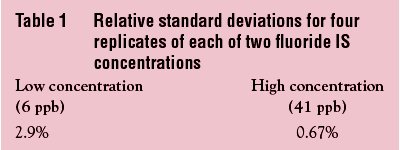
To evaluate precision, a combined experiment was conducted. Both low (6 ppb) and high (41 ppb) fluoride concentrations were chosen. (The selected concentrations were lower than the bottom and top of the analyte range, since the ion-chromatographic response per unit mass of fluoride is higher than are the ratios for the other analytes.) For the calibration study involving the analytes, a 10-concentration design was used (i.e., blank; 12, 15, 18, 21, 24, 29, 35, 41, and 47 ppb). This suite of standards was prepared (in deionized water) and analyzed on each of eight separate days. The low and high levels of fluoride were added on alternating days, yielding four data sets for each IS concentration. The precision results for the two fluoride levels are shown in Table 1. The RSD for the high concentration was roughly 45 times less than the corresponding value for the low concentration. Thus, 41 ppb was chosen as the preferred IS concentration.
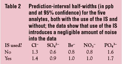
The data sets that involved the 41 ppb of fluoride were used to construct the two calibration curves (i.e., scaled and unscaled) for each analyte. Prediction intervals (at 95% confidence) were compared (see Table 2). Use of the IS added only 0.1–0.3 ppb to the half-width of each analyte’s prediction interval; this amount was deemed to be negligible. Thus, an IS of 41 ppb fluoride was acceptable from the standpoint of precision.
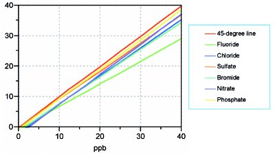
Figure 1 - Overlay plot showing the SL/OLS recovery curves for the five analytes and fluoride. Also shown (in red) is the 45-degree line, which represents 100% recovery.
To evaluate recoveries, the following spiking study was conducted. From a stock standard (containing all five analytes and fluoride), nine concentrations (blank; 10, 12.5, 15, 17.5, 20, 25, 30, 35, and 40 ppb) were prepared in 30% hydrogen peroxide. (These levels were slightly different from the pure-water calibration study above, since H2O2 loses mass when it is digested.) This suite of spiked samples was prepared, digested, and chromatographed on each of eight separate days. The predicted concentrations of each anion were calculated using the unscaled calibration curves above. After adjusting for any positive blanks, the recovered amounts were plotted vs true concentration. An overlay of all six resulting SL/OLS curves is seen in Figure 1; also shown is the 45-degree line, which represents 100% recovery. The slope of each anions’ line reflects the percent recovery.
With one exception (i.e., the green line), all slopes appear to be similar, and at or above roughly 90%. The identity of the “odd man out” is fluoride! Clearly, the recovery for this IS candidate does not mimic that of any analyte. Furthermore, a closer look at Figure 1 show that all curves have a negative intercept. This feature indicates that there is a constant bias, which cannot be offset by an internal standard (since an IS can only correct for proportional problems). An alternative solution to “recovery-plagued” methods will be discussed in the next installment.
Mr. Coleman is an Applied Statistician, Alcoa Technical Center, MSTC, 100 Technical Dr., Alcoa Center, PA 15069, U.S.A.; e-mail: [email protected]. Ms. Vanatta is an Analytical Chemist, Air Liquide-Balazs™ Analytical Services, Box 650311, MS 301, Dallas, TX 75265, U.S.A.; tel.: 972-995-7541; fax: 972-995-3204; e-mail: [email protected].