In the previous article (American Laboratory Aug 2005), borate data were presented. No single model was found to be adequate. Thus, the alternative of dividing the concentration range into intervals was proposed. This installment will discuss the segmenting process and develop a calibration curve for the data in each region.
The first task is to decide how the data should be divided. The resulting subsets should be such that two criteria are met. First, there must be sufficient concentration levels and replicates to allow for meaningful calibration diagnostics. Second, there should be evidence that a single (and preferably simple) model can explain the data in each interval.
The most helpful tool in this process is residual analysis (i.e., the search for patterns in the residuals, or other departures from random behavior). Three models (i.e., straight-line, quadratic, and cubic, each with weighted-least-squares fitting) were tested in the previous article. The residual patterns were quite similar; the one for the straight line is shown in Figure 1.
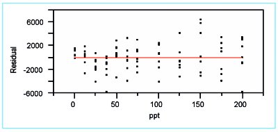
Figure 1 - Residuals plot for a straight-line fit (with weighted-least-squares fitting) to the borate data.
From the appearance of this pattern, a possible dividing point might be between 37.5 and 50 ppt. However, such a decision results in only four levels in the lower range. A better dividing point would be 75 ppt. The logic is as follows. The data for the range of 0–75 ppt show curvature (i.e., the pattern trends downward through 37.5 ppt and then moves back up). This approximately parabolic shape suggests that a quadratic model might be appropriate for this region. The remaining data (i.e., 100–200 ppt) exhibit a fairly random scatter about the zero line, indicating a straight-line model might be adequate for this upper range.
Since the data points for 75 ppt appear random about zero, they can be included in the second data set as well as the first. This "doubling up" creates a "bridge" between the two calibration curves that will be developed. This scheme also satisfies the first criterion mentioned above; the lower range has seven levels and the higher region has six. Also, each level has eight replicates.
Calibration diagnostics for the lower concentration range: 0–75 ppt
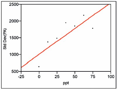
Figure 2 - For the lower concentration range, plot of the standard deviations of the responses vs concentration. Since the slope's p-value (0.0227) is above 0.01, OLS is an appropriate fitting technique.
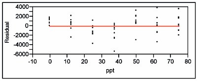
Figure 3 - Residual pattern and lack-of-fit p-value for an SL/OLS fit of the lower-range borate data. These diagnostics show that a straight line is not an adequate model.
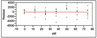
Figure 4 - Residual pattern and lack-of-fit p-value for a quadratic model fit (with OLS) to the lower-range borate data. Indications are that this model is adequate.
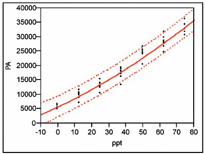
Figure 5 - Regression line and prediction interval (at 95% confidence) for the quadratic model fit to the lower-range data via OLS.
When the standard deviations of the responses are plotted vs concentration, the straight-line/ordinary-least-squares (SL/OLS) curve has a slope p-value of 0.0227, which is above the cutoff of 0.01 (see Figure 2). Thus, OLS is an appropriate fitting technique for the response-vs-concentration data themselves. A SL is then fitted to the data using OLS. The residual pattern and lack-of-fit p-value are presented in Figure 3. The pattern exhibits curvature, and the p-value (0.0072) indicates the model is not adequate. When a quadratic model (also with OLS fitting) is tested, the results are much improved (see Figure 4). The residuals are closer to random about the zero line, with the qualifier that there still appears to be a break between 37.5 and 50 ppt. However, the lack-of-fit p-value (0.0645) is above the 0.05 cutoff. (If a cubic model is tested, the cubic term's p-value [0.2024] is not significant, since it is well above the 0.01 cutoff. This finding provides further evidence that a quadratic model is adequate.)
The appropriate calibration line and its prediction interval (at 95% confidence) are shown in Figure 5. Because the response standard deviation is constant over the concentration range, the prediction-interval width is approximately the same throughout the calibration range.
Calibration diagnostics for the higher concentration range: 75–200 ppt
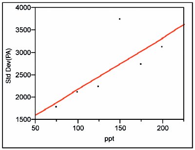
Figure 6 - Standard deviations of the responses plotted vs true concentration for the higher range.
The standard deviations of the responses are modeled first, again with a SL model using OLS fitting (see Figure 6). The standard deviation for the 150-ppt data appears to be out of line with the other values. There is a possibility that at least one of the raw data points is corrupted. However, the peak-area values were 58795, 61479, 58211, 60605, 65462, 60648, 67655, and 67183; nothing other than random noise is apparent; thus all of the data are accepted. The p-value for the slope is 0.0891, which indicates that the slope is insignificant.
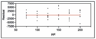
Figure 7 - Residual pattern and lack-of-fit p-value for the SL model (with OLS fitting) applied to the higher-range borate data.
As a result, OLS is the appropriate fitting technique for these response-vs-concentration data. A SL model (with OLS fitting) is tested first. The residual pattern and lack-of-fit p-value are shown in Figure 7. The residuals are scattered fairly randomly about the zero line. Furthermore, the lack-of-fit p-value is 0.7428, indicating that the model is adequate. (Additional confirmation of this decision comes from fitting a quadratic model with OLS fitting. The p-value for the quadratic term is insignificant at 0.8930. Thus, use of a higher-order polynomial would result in overfitting the data.)
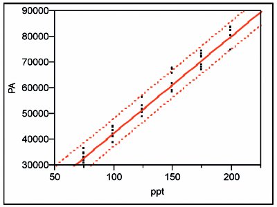
Figure 8 - SL/OLS curve and prediction interval (at 95% confidence) for the higher-range data.
The SL/OLS curve (with its 95%-confidence prediction interval) is shown in Figure 8. As with the lower-range curve, OLS fitting is appropriate, and thus the width of the prediction interval is approximately constant over the entire range.
Remaining issues
Once the above curves have been developed, statistical analysis of these data is complete. However, several questions remain. First, is it acceptable to the user to have two calibration curves for the data? Second, are the prediction intervals tight enough for the situation at hand? Third, are these curves and intervals more reliable and more useful than the single curve and interval that were developed in the previous installment? Fourth, should additional constraints be imposed at 75 ppt? For example, should there be forced agreement in one or more of the following: the predicted concentration, the calibration-line slopes, or the widths of the confidence interval? Depending on the answers to these questions, the user may have to conduct a more detailed calibration study and subsequent statistical analysis.
Mr. Coleman is an Applied Statistician, Alcoa Technical Center, MSTC, 100 Technical Dr., Alcoa Center, PA 15069, U.S.A.; e-mail: [email protected]. Ms. Vanatta is an Analytical Chemist, Air Liquide-Balazs™ Analytical Services, Box 650311, MS 301, Dallas, TX 75265, U.S.A.; tel.: 972-995-7541; fax: 972-995-3204; e-mail: [email protected].