This installment will present the sixth and last in this series of calibration examples. The data again are from an ion chromatographic calibration experiment; the analyte was borate. Since the calibration design has not been discussed previously, it is described here. The concentration range of interest was from 0 ppt (i.e., a blank) to 200 ppt; a low detection limit was desired as well as reliable predictions along the entire concentration range. Thus, the following 12 levels were chosen: a blank; 12.5, 25, 37.5, 50, 62.5, 75, 100, 125, 150, 175, and 200 ppt. These standards were prepared and chromatographed on eight separate days. Responses were measured in units of peak area (PA). Since this analyte had not been tested previously, no data were available to help suggest a model. Thus, a straight-line model, fit with ordinary least squares (OLS), was proposed. Once the 96 data points were available, the calibration diagnostics were begun.
Step 1: Plot response vs true concentration
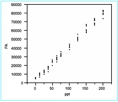
Figure 1 - Scatterplot of the borate responses versus true concentration. No errant data points are detected.
The scatterplot (Figure 1) shows no errant points, but does suggest that the response variation may be increasing with concentration. Also, there may be slight curvature to the data.
Step 2: Determine the behavior of the standard deviation of the response
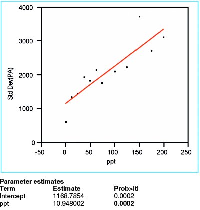
Figure 2 - Plot of standard deviation of responses versus true concentration. The low p-value (in boldface) for the slope indicates that the standard deviation changes with concentration.
In order to evaluate the response variation, the standard deviation of the responses is calculated for each concentration, and then plotted versus the true concentration. When a straight line is fitted to these data, using OLS fitting, the p-value for the slope is seen to be 0.0002 (Figure 2). This value is significant, meaning that the starting hypothesis (i.e., a straight line with zero slope plotted through the mean of the data) is not a good model (i.e., should be rejected). Instead, a line with a positive slope is accepted. This positive slope means that the variation does increase with concentration; therefore the proposed fitting technique (i.e., OLS) is not appropriate for these response-vs-concentration data. Instead, weighted least squares (WLS) is needed. Weights are calculated according to the formula discussed in Part 8 (American Laboratory, Nov 2003) and applied to all future modeling of the peak-area data. Note that over the span of the concentration range, Figure 2 shows an approximately threefold increase in standard deviation; the implication is that there is an approximately ninefold decrease in relative weights of “noisy” data to “precise” data (since weights are proportional to the reciprocal square of the standard deviation).
Steps 3–6: Fit the proposed model; evaluate R2adj, residual pattern, slope’s p-value, and lack-of-fit p-value
As occurred with the previous example (American Laboratory, Feb 2005), more than one model will need to be considered. Thus, steps 3–6 will be used iteratively and as a group.
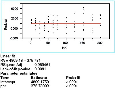
Figure 3 - Results from a straight-line model fitted to the borate data, using WLS as the fitting technique.
Now that the fitting technique has been determined, the straight-line model is fitted to the data. The summary statistics and residuals are shown in Figure 3. At 0.989, R2adj is sufficiently high, especially since this diagnostic tool is not a particularly strong indicator of model appropriateness.
The residuals are not as random as would be anticipated for adequate model selection. For the first four concentrations, the residual means trend downward. The clusters at 100 and 150 ppt “ride” low and high, respectively. Thus, the proposed model may be lacking one or more terms.
The p-value for the slope is less than 0.01. Therefore, as expected, a straight-line model is a better choice than is the starting hypothesis (i.e., a zero-slope line through the mean of the data points). However, a statistically significant slope does not, by itself, indicate that the straight line is an adequate model.
The lack-of-fit p-value is 0.0081, thereby confirming the postulation from the residual pattern. Since the starting hypothesis for this test is that there is no lack of fit, the low result for the proposed model means that the model is not adequate.
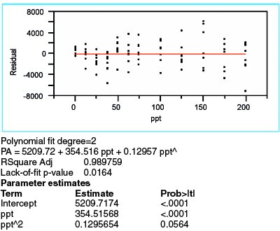
Figure 4 - Data for a quadratic model, with WLS fitting, applied to the borate data.
After rejecting the straight-line model, a logical choice is a quadratic. The results are shown in Figure 4 (using WLS fitting, since the choice of fitting technique depends solely on the behavior of the standard deviations of the responses). There are still signs of model inadequacy. First, the residual pattern once again appears to be nonrandom. The clusters for the first four concentrations continue to trend downward. Second, the lack-of-fit p-value (0.0164), while higher than with the straight-line model, is still below the recommended cutoff of 0.05. Finally, the p-value (0.0564) for the quadratic term is not statistically significant (albeit not too far above the typical cutoff of 0.01). Hence, adding a quadratic term may not be sufficient to effect an adequate model.
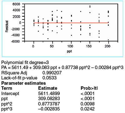
Figure 5 - Regression outcome for a cubic fit (with WLS fitting) of the borate data.
Because there is evidence (i.e., residual pattern and lack-of-fit p-value) that the quadratic model is not adequate and because the quadratic-term p-value is borderline, it is appropriate to investigate the cubic model. The WLS results for a third-order polynomial are shown in Figure 5. The cubic term's p-value (0.0242) is only barely insignificant. However, the lack-of-fit p-value is borderline, since 0.05 is the traditional cutoff. Most telling of all is the residual pattern, which continues to display a trend in the lower-concentration range.
Inadequate-model evaluation
At this stage, it is clear that no simple polynomial model can explain these data in a statistically sound manner. The next step is to determine what “penalty” will be paid if one of the inadequate models is selected. The procedure is the same as was detailed in the previous article (American Laboratory, May 2005).
As with the earlier example, a quadratic model (with the necessary WLS fitting) was chosen, since it can be inverted easily via the quadratic formula. The goal is to determine the uncertainty that results from using this less-than-adequate (i.e., biased) model. This variability is over and above the random uncertainty that is captured by the prediction interval. This bias contribution (at 95% confidence) can be approximated by determining (at each concentration) the quantity:
(mean residual) ± 2 * (standard error of the mean residual).
This error interval is combined with the prediction interval (also at 95% confidence) to give the overall uncertainty (i.e., random plus bias) for the calibration line; the confidence level for this total uncertainty is ~90%.
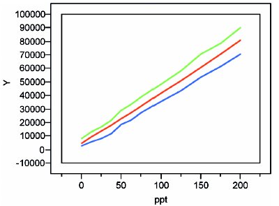
Figure 6 - Quadratic plot with precision-plus-bias prediction interval (~90% confidence).
The result for these borate data is shown in Figure 6. Except at low concentrations, the two envelope lines are roughly parallel to and equidistant from the calibration line. For concentrations below ca. 75 ppt, the “waviness” of the limits is a concern. The uncertainty envelope changes markedly and quickly as one moves up and down the concentration scale. Thus, the uncertainties reported between 12.5 and 75 ppt will not be very reliable, and one of the goals (see paragraph 1) of this study will not be met.
It is possible that these data cannot be explained adequately with one model. A potential solution would be to divide the concentration range into intervals (in this case, probably two in number) and generate a calibration curve for each data subset. This alternative will be discussed in the next installment.
Mr. Coleman is an Applied Statistician, Alcoa Technical Center, MST-C, 100 Technical Dr., Alcoa Center, PA 15069, U.S.A.; e-mail: [email protected]. Ms. Vanatta is an Analytical Chemist, Air Liquide-Balazs™ Analytical Services, Box 650311, MS 301, Dallas, TX 75265, U.S.A.; tel: 972-995-7541; fax: 972-995-3204; e-mail: [email protected].