In the previous article (American Laboratory, Feb 2005), calibration data were diagnosed for a study involving phosphate. The concentration range was from 1 to 98% (wt/wt); response data were in units of peak area (PA). The evaluation revealed that a cubic model with weighted-least-squares (WLS) fitting was appropriate. However, a cubic (or any higher-order polynomial) model has the practical disadvantage of being difficult to invert for prediction purposes. The possibility was offered of using a simpler model (i.e., quadratic) if it was found to provide adequate information (i.e., acceptably low uncertainty). Use of this model, however, would involve estimation not only of precision but also of bias, since the model displayed statistically significant lack of fit. The current column addresses a procedure for estimating both precision and bias, and for seeing the consequences of using an under-fitting model (i.e., a model with bias, which is evidenced by a statistically significant p-value for the lack-of-fit test).
The development of an estimation procedure involves discussion of root mean square error (RMSE). In general, RMSE is related to precision and bias as follows:
(RMSE)2 = Variance + (Bias)2.
Thus:
where Variance is the variance of the response (i.e., the variance is the square of the standard deviation). As was seen in Part 4 (American Laboratory, Mar 2003), the width of uncertainty intervals is proportional to RMSE. Since only precision should be involved in prediction-interval calculations, RMSE should not include a bias term. Under the assumption that an adequate model has been selected for calibration, the bias term can be equated to be zero. However, for an under-fitting model, bias is present. Even though all of the bias is captured in RMSE, the prediction interval does not inflate enough (and in the right places) to incorporate all of the bias. Furthermore, the prediction interval cannot reflect the effects of bias that changes with concentration. Nevertheless, the precision and bias components for an under-fitting model can be approximately extracted and illustrated. In the remainder of this article, this process will be demonstrated for the quadratic/WLS model fitted to the phosphate data.
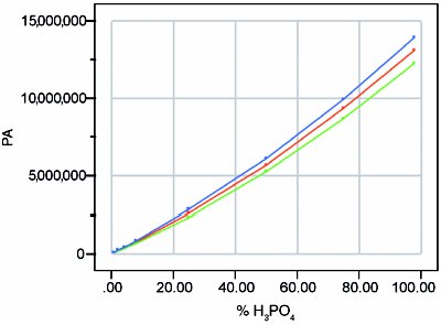
Figure 1 - Quadratic-model fit by WLS, with 95%-confidence uncertainty envelope (i.e., prediction interval) for a single future measurement.
Figure 1 shows the quadratic-model fit (by WLS) with its 95%-confidence uncertainty envelope (i.e., prediction interval) for a single future measurement. Given that a correct decision was made regarding response variation (i.e., that it increases with increasing concentration), Figure 1 appears to depict a typically shaped interval for data with nonconstant standard deviation of the response. However, the uncertainty interval is misleading, since the measurement is encumbered by systematic bias as well as random response variation.
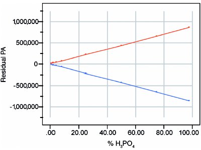
Figure 2 - Prediction interval (at 95% confidence and based on the quadratic-model fit by WLS) after subtracting out the calibration line.
Figure 2 displays the increase in the vertical separation of the 95%-confidence prediction interval with increasing concentration. The plot is residual in nature, since it was generated by subtraction (here, by subtracting the calibration line from both the upper prediction limit and the lower prediction limit). This interval reflects all of the random uncertainty and some of the bias. The interval is also symmetric in PA, and is approximately symmetric in concentration.
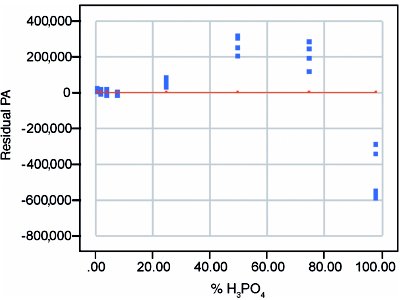
Figure 3 - Residuals from quadratic-model fit by WLS. The plot reveals bias that changes with concentration.
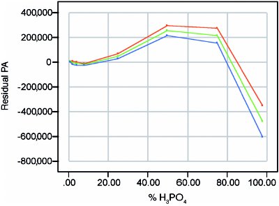
Figure 4 - Plot of estimated bias (center line) along with the uncertainty envelope (at 95% confidence) for the bias.
To estimate bias correctly (and the uncertainty associated with it), the residual plot itself (Figure 3) is used, since residuals are the true minus the predicted. The bias is estimated by computing the mean residual at each concentration. These values are then plotted versus true concentration. Since these bias values are estimates, they have uncertainty. At each concentration, that uncertainty is approximated by the standard error of the bias mean. A plot of two times these bias standard errors will generate a 95%-confidence uncertainty interval for the bias curve. (For normal curves, two standard deviations represent approximately 95% of the distribution.) The overall plot for bias (showing the bias itself as well as its uncertainty interval) is seen in Figure 4. As with the residual plot itself, the estimated bias is small (in absolute terms) for low concentrations, positive for midlevel concentrations, and negative for high concentrations.
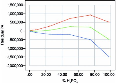
Figure 5 - Graph showing combined uncertainties. The center line reflects bias plus precision. The combined uncertainty envelope is at an overall confidence level of ~90%.
Figures 2 and 4 can be combined into one residual-type plot (Figure 5) that estimates the combined uncertainty (i.e., the uncertainty from noise plus the uncertainty in bias). The merging process is as follows. At each concentration, the widths of the upper limits (from Figures 2 and 4) are added together; the widths of the lower limits are added together similarly. The two new limits are then plotted versus true concentration, as is the bias line from Figure 4 (the center line for Figure 2 is zero, since the calibration line has been subtracted out at each concentration). The combining of two 95%-confidence intervals into one generates a new envelope that has a confidence level of ~90%. The vertical scale of Figure 5 (and of all residual-type plots) allows the intervals' shapes to be seen in detail.
Figure 6 - Calibration curve (center line) from Figure 1, along with the rescaled uncertainty envelope from Figure 5.
Ultimately, though, the graph that is desired is seen in Figure 6. This final plot is on the same scale as the calibration curve (with its prediction interval) seen in Figure 1. Indeed, the center line of Figure 6 is the calibration (i.e., center) line from Figure 1. However, in this last plot, each uncertainty limit has the width seen in Figure 5. In other words, the calibration line has been added back into Figure 5. The result is a graph that is useful for predicting samples and for reporting such data along with an appropriate uncertainty. Note that the interval is not symmetric.
It should also be noted that the widths seen in both Figures 5 and 6 overstate bias at least slightly. Figure 4 estimates all of the bias. However, as was stated earlier, the prediction interval (shown in Figure 1) is inflated somewhat because bias is not zero in the RMSE term of the prediction–interval formula. Unfortunately, there is no way to determine how much of the prediction interval's width is due to bias (although it is not trivial, by comparison to the ~50% lower RMSE from a cubic fit; American Laboratory, Feb 2005). Thus, there is some "double counting" in the final interval seen in Figure 6.
If the intervals in Figures 1 and 6 are compared, there is very little difference between the two. This observation may lead the reader to think that the above procedure was only a didactic exercise with few practical implications. Such is not the case; just because this example did not show a large effect from bias does not mean that all data sets will behave similarly. In fact, if the user had decided to use the straight-line fit for these phosphate data, the bias-plus-precision plot would have displayed a large envelope at high concentrations. In the end, the overall recommendation is that the reader realize that there are serious tradeoffs to be weighed when considering the use of an inadequate model. In this current example, the quadratic model is simpler than the cubic model and is easier to invert (the quadratic formula is much more tractable than the cubic equations). However, the second-order polynomial also shows statistically significant lack of fit, thereby leading to both bias and precision problems that are difficult to characterize. On the other hand, the cubic model has an additional term that makes it difficult to invert by formula. However, it has no evidence of lack of fit, and hence no evidence of systematic bias; the prediction interval can be trusted to represent uncertainty, and a look-up table or iterative procedure can be used instead of an inverse formula.
In the end, only the user(s) can decide if statistically significant results are practically important. Only if the data have been diagnosed in a statistically sound manner will reliable results be available for making such decisions.
Mr. Coleman is an Applied Statistician, Alcoa Technical Center, MSTC, 100 Technical Dr., Alcoa Center, PA 15069, U.S.A.; e-mail: [email protected]. Ms. Vanatta is an Analytical Chemist, Air Liquide-Balazs™ Analytical Services, Box 650311, MS 301, Dallas, TX 75265, U.S.A.; tel: 972-995-7541; fax: 972-995-3204; e-mail: [email protected].