This real-world example of calibration diagnostics involves the ion-chromatographic behavior of phosphoric acid; phosphate is the actual analyte form that is measured by the instrument. The chemical was part of a statistically designed mixture experiment where each component could vary from 1 to 98% (wt/wt). The calibration design was discussed in Part 6 (American Laboratory, Jul 2003). Eight standards (i.e., 1, 2, 4, 8, 25, 50, 75, and 98%) were each analyzed five times. Phosphate typically exhibits straight-line behavior for peak area (PA) vs concentration; thus, that type of model was proposed for the data, using ordinary least squares (OLS) as the fitting technique.
Step 1: Plot response vs true concentration
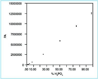
Figure 1 - Scatterplot for the phosphate data.
In Figure 1, the response data are plotted vs true concentration. No outliers or other “errant” points are visible. However, a distinct concave shape is seen in the graph, indicating that a straight line might not be the appropriate model for these data. Also, some of the points at higher concentrations appear to be noisier than do most of the points at lower concentrations. These observations will be evaluated more rigorously via the following diagnostics.
Step 2: Determine the behavior of the standard deviation of the response
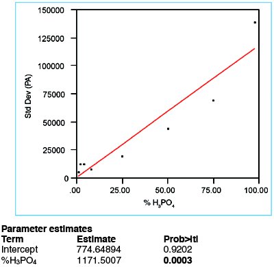
Figure 2 - Plot of response standard deviation vs true concentration; data have been fitted with a straight line, using OLS as the fitting technique.
In Figure 2, the responses’ standard deviations are plotted vs true concentration and fitted with a straight line, using OLS fitting. The p-value for the slope is only 0.0003 (boldfaced in Figure 2), which is well below the typical cutoff of 0.01. Thus, the slope is significant and the standard deviation is deemed to be nonconstant. Therefore, weighted least squares (WLS) should be used as the fitting technique, not OLS. This decision gives statistical confirmation of the increasing-noise suspicion raised via visual inspection in step 1.
To determine the weights for use in WLS fitting, the response’s standard deviation (SD) is predicted using the parameter estimates given in Figure 2 (i.e., SD = 774.64894 + [1171.507 * %H3PO4]). Each weight is the reciprocal square of this formula, divided by the mean of all these reciprocal squares.
Steps 3–6: Fit the proposed model; evaluate R2adj, residual pattern, slope’s pvalue, and lack-of-fit p-value
The alert reader will notice that in this article, discussion of the next four steps has been combined into one heading. This example is more complicated than the previous four, and will involve the examination of several models. Thus, these steps will have to be used iteratively and, for clarity, will be taken as a group.
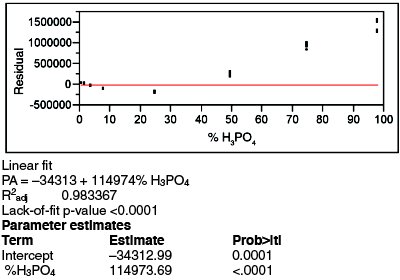
Figure 3 - Residuals pattern and regression statistics for a straight-line fit of the data, using WLS (PA-vs-concentration plot not shown). The distinct pattern in the residuals plot indicates that this model is inadequate for these data.
To begin, the proposed straight-line model is fitted. Since the proposed fitting technique (i.e., OLS) was rejected in step 2, WLS is used instead. The residuals plot and regression statistics are shown in Figure 3. R2adj is only 0.9834, but since this statistic is a relatively weak indicator of model appropriateness, the value does not signal an alarm. However, the residual pattern veritably screams that there is a problem; there is nothing random about this pattern. As expected, the p-value for the slope is <0.01, meaning that a straight line is a better model than the starting hypothesis (which is that an adequate model is a straight line, with slope = 0, through the mean of each concentration’s data). However, this low value in and of itself does not indicate that a straight line is adequate. To the contrary, the lack-of-fit p-value is <0.0001, well below the customary 0.05 cutoff. Since the starting hypothesis for this test is that there is no lack of fit for the proposed model, such a calculated value means that the proposed straight line is not appropriate.
The lack-of-fit test does not help in selecting a model better than one that fails. However, the residuals plot does afford clues. The shape seems to be somewhere between a parabolic and a cubic pattern.
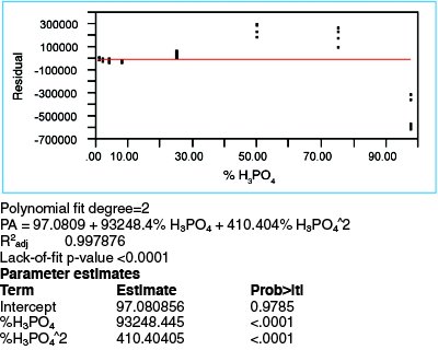
Figure 4 - Residuals plot and regression statistics for a quadratic fit, with WLS fitting. This residuals plot also exhibits a distinct pattern.
A quadratic model (with WLS fitting, per step 2) is tried first. The residuals plot and regression statistics are shown in Figure 4. R2adj has risen to 0.9979, weakly confirming that the additional term does not result in overfitting. The p-value (<0.0001) for the quadratic term (see “%H3PO4^2” term under “Parameter estimates”) also means that adding this term is appropriate. However, the residuals plot still exhibits an undulating pattern and the lack-of-fit p-value is still <0.0001. Thus, there is still an inadequacy-of-model problem.
The next step in complexity is to try a cubic fit. Whenever this situation occurs, though, it is best to proceed with caution. First, if a third-order polynomial is found to be adequate, it may be difficult to invert the equation (x as a function of y, rather than y as a function of x), since not all software packages automatically perform this operation. Yet this inversion is needed when using a calibration curve to calculate concentrations for unknown samples. Regressing x on y is not an acceptable procedure to overcome this difficulty (see Part 3, American Laboratory, Jan 2003). More importantly, the need for higher-order polynomials often suggests that the concentration range is too wide to be explained adequately by one model; breaking up the range and performing piecewise calibration may be more appropriate.
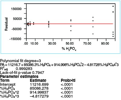
Figure 5 - For a cubic fit, with WLS fitting, the residuals plot is fairly random about zero. The lack-of-fit p-value is above the recommended 0.05 threshold. Both observations indicate this model is adequate.
Thus, with these caveats in mind, a cubic model is evaluated using WLS. As seen in Figure 5, R2adj has now risen to 0.9993; the p-value for the “%H3PO4^3” term is <0.0001, meaning that the term is statistically significant. The residuals appear fairly random, with the zero line’s going approximately through the mean of the data at each concentration. Lastly, the lack-of-fit p-value of 0.7947 is well above the 0.05 cutoff. Thus, all indications are that this model is adequate and thus a better choice (statistically) than either a straight-line or quadratic fit.
Step 7: Plot and evaluate the prediction interval
By now, the statistical questions have been answered and the statistical decision made (i.e., a cubic fit is an appropriate model for these data). Practical considerations remain. The concentration range of 1–98% probably is too wide to be handled well with only one model. As discussed above, it might be better to break up the range into segments, include additional concentration standards as needed, and determine a separate calibration curve for each region. The question that arises immediately is, “Is all that extra work worth the effort, time, and money?” For this study, a calibration curve was needed to determine the concentration of reaction products in a statistically designed mixture experiment. Knowing the amount to within a few percentage points (absolute) was sufficient; if a less-than-adequate (but simpler) model provided adequate information, it would suffice. (In Part 3, American Laboratory, Jan 2003, statistician George Box was quoted as saying, “All models are wrong; some are useful.”)
The next step would be to reevaluate the quadratic model (using WLS) and its prediction interval. However, since the quadratic model showed a lack of fit, there is not only an uncertainty issue but a systematic-bias problem. For the various regions of the working range of concentrations, estimations of both precision and bias must be made. These procedures will be addressed in the next column.
Mr. Coleman is an Applied Statistician, Alcoa Technical Center, MSTC, 100 Technical Dr., Alcoa Center, PA 15069, U.S.A.; e-mail: [email protected]. Ms. Vanatta is an Analytical Chemist, Air Liquide-Balazs™ Analytical Services, Box 650311, MS 301, Dallas, TX 75265, U.S.A.; tel: 972-995-7541; fax: 972-995-3204; e-mail: [email protected].