It is possible to associate a relative standard deviation or the more general relative measurement uncertainty (RSD and RMU, respectively) with a detection limit (DL). (Note: For details on the detection-limit material presented here, see the following American Laboratory articles in this series: Parts 28–30, Nov/Dec 2007, Feb 2008, and Jun/Jul 2008, respectively; Parts 32 and 33, Nov/Dec 2008 and Mar 2009, respectively.) However, the linkage can lead to confusion. This article will look at the problems that can arise. The discussion begins with a categorization of these limits.
DLs are an interesting statistic in that many formulas have been proposed for calculating the limit, but there remains a good deal of debate as to which procedure is “correct” or “best.” Suffice it to say that most all such protocols fall into one of two bins: 1) only the rate of false positives (i.e., alpha or α) is controlled or 2) both the rate of false positives and the rate of false negatives (i.e., beta or β) are controlled. The relative uncertainty that can be associated with a given DL will depend in part on which of the two categories is appropriate.
Consider type 1. Typically, such a DL is some multiple of the sample standard deviation (s) of replicate blank measurements; the multiplier (t) is the value of Student’s t for the confidence level chosen and the number of degrees of freedom available. In this situation, the RSD is appropriate. Recall from the previous article (American Laboratory, Jun/Jul 2012) that a generally accepted definition of RSD is, “The standard deviation (s) of a set of data, divided by the mean (xavg) of the data set, expressed as a percentage.” Thus, the formula is:
RSD = (s ÷ xavg) * 100% (1)
In the case of a type-1 DL, Eq. (1) becomes:
RSD = (s ÷ DL) * 100%, or (2)
RSD = [s/(t*s)] * 100%, or (3)
RSD = 100%/t (4)
since s is being compared with the calculated DL, not with the mean of the data set. This reality means that the RSD is a ratio of two dependent values, s and t*s. (With typical RSDs, the mean and the standard deviation are assumed to be independent of each other.) As a result, the RSD associated with a type-1 RSD will depend only on the value of Student’s t.
Since low-level standards can also be used to generate this type of DL, the value of the limit typically will vary, depending on the level chosen. This phenomenon is seen especially in situations where s trends (typically higher) with increasing concentration (i.e., where s is dependent on the concentration). In addition, s is a very noisy statistic; even if the standard deviation does not trend, the calculated DLs may differ among the various standards used to generate the limit. Nevertheless, because of the dependent nature of Eq. (3), the same RSD will be associated with each different DL that is possible for a given data set (i.e., the RSD will still depend only on the value of t).
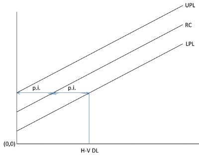
Figure 1 – Graph depicting the relationship between the half-width of the prediction interval and a Hubaux-Vos DL; see text for details. Acronyms: 1) UPL = upper prediction limit, 2) RC = regression curve, 3) LPL = lower prediction limit, 4) p.i. = half-width of prediction interval in concentration units, 5) H-V DL = Hubaux-Vos DL in concentration units.
Three realities should be emphasized, relative to type-1 DLs. First, Student’s t is the proper multiplier, not the z-score associated with a Normal curve. An assumption of Normal curves is that the underlying data are “truth.” In the real world, all measurements are estimates, meaning that the t-distribution should be used.
Second, unlike z-scores, the value of Student’s t does not depend solely on the value of α. The available degrees of freedom (dof, related to the number of data points and therefore the number of replicates analyzed) also influence t-values. Especially if the number of dof is low (i.e., less than 6 or 7), Student’s t will rise rapidly as the dof decline. Thus, the RSD will fall accordingly.
Third, with type-1 DLs, all of the uncertainty (i.e., α) is in one tail of the t-distribution. Thus, two-tail linkages between confidence level and number of standard deviations may not approximate reality.
Now consider the type-2 DL. Here, the calculation becomes more complicated, since both α and β are being controlled; the estimate of s is multiplied not only by t, but also by another expression, which will depend on the protocol being used. In these instances, RMU is the appropriate statistic.
One type-2 protocol was detailed by Hubaux and Vos. In their formula, the ± measurement uncertainty includes not only t and s, but also the formula for the prediction interval’s half-width (p.i.). (See Part 4, American Laboratory, Mar 2003, for details on prediction intervals and their formula.)
As was explained in earlier articles, the Hubaux-Vos (H-V) DL can be determined graphically, as shown in Figure 1. For a specific pair of α and β values, only one HVDL will result for a given data set.
If α = β, then (to a close approximation) the H-V DL is twice the half-width of the prediction interval. Thus, the RMU is:
RMU = [p.i./(2 * p.i.)] * 100% (5)
The RMU for the H-V DL is independent of confidence level and is always equal to 50%, if α = β.
If α ≠ β, then the determination of the RMU actually does not make sense. In such cases, the prediction interval is not symmetric, so Eq. (5) does not apply. The only possibility would be to calculate two RMUs, using the “positive” half-width of the prediction interval and the “negative” half-width, in turn. Such results would not be useful in the practical world.
As its name implies, a prediction interval reports the uncertainty in the next measurement (i.e., instrument response) that is converted to concentration units via the regression curve that is being used. DLs are calculated for application to future samples and check standards whose concentrations are being estimated, using the appropriate curve. Since type-1 DLs rely solely on the standard deviation of replicate measurements at one concentration, this statistic (or the related RSD) does not speak to future measurements. Instead, an RMU of the type described above is needed.
Is it possible to calculate the RMU associated with a type-1 DL, using the H-V approach? In reality, the answer is “no.” With such a limit, α ≠ β, meaning that such a calculation is not useful; see above discussion.
What is the take-home message from the above? Be very careful when discussing detection limits in terms of relative uncertainties. It is common to report only the DL and the magnitude of any associated uncertainty (absolute or relative) that has been calculated. However, this information alone does not give the recipient the ability to understand how the values were determined, and whether an RSD or RMU is the actual statistic that has been chosen.
An even better suggestion is to abandon DL-Land completely. Instead, do a thorough, statistically sound job of determining the analytical method’s overall uncertainty. Then report: 1) concentration results, 2) overall uncertainty, and 3) the associated confidence level that has been chosen.
David Coleman is an Applied Statistician, and Lynn Vanatta is an Analytical Chemist; e-mail: [email protected].